ClickHouse is best known as an analytics engine built for speed at scale, but over the past several years it has grown a surprisingly complete set of geospatial capabilities.
In this post we're going to take a tour of where things stand today: the type system, the functions, the sharp edges, a look at where ClickHouse fits and where it does not.
A brief history #
Geospatial support in ClickHouse has grown steadily over time rather than arriving all at once.
ClickHouse uses a YY.MM versioning scheme - version 20.1 shipped in January 2020, 21.9 in September 2021, and so on. The earliest geospatial functions predate this scheme and appear under version 1.x in the function catalog.
Those early functions were a handful of coordinate-distance functions: greatCircleDistance and eventually geoDistance. There were no geometry types - functions just took raw coordinate values as parameters.
In 2020 (version 20.1), the grid-based indexing systems arrived: geohashEncode/geohashDecode and H3 (Uber's hexagonal hierarchical grid) both landed in that release. S2 (Google's spherical geometry library) followed in 2021 (version 21.9). These cover a huge share of real-world spatial analytics use cases - binning observations into cells, aggregating by region at a chosen resolution, proximity lookups - and ClickHouse handles them extremely fast.
Point, Ring, Polygon, and MultiPolygon arrived in v20.5 (May 2020), initially behind an experimental flag. They are custom names layered over ClickHouse's existing primitives - Tuple and Array - rather than a separate storage format. The experimental flag was removed in v23.5, making them production-ready. WKT parsing functions like readWKTPolygon and svg followed in v21.4. LineString came later still, added in v24.6.
The most significant recent additions both landed in 2025. The Geometry type, introduced in v25.11, uses the Variant type and can hold any geometry subtype in a single column - points alongside polygons alongside linestrings - without splitting into separate columns or tables. WKB (Well-Known Binary) support arrived around the same time (v25.7–v25.12), enabling direct import from PostGIS and other GIS tools without a text parsing round-trip.
If you want to trace this history yourself, you can use the system.functions table, which records which version each function was introduced in:
1SELECT
2    splitByChar('.', introduced_in)[1] AS major_version,
3    count(),
4    bar(count(), 0, 40, 40) AS chart
5FROM system.functions
6WHERE categories LIKE '%Geo%'
7GROUP BY major_version
8ORDER BY major_version ASC
┌─major_version─┬─count()─┬─chart───────────────────────────────────┐
│ 1             │       5 │ █████                                   │
│ 20            │      17 │ █████████████████                       │
│ 21            │      39 │ ███████████████████████████████████████ │
│ 22            │      23 │ ███████████████████████                 │
│ 25            │      15 │ ███████████████                         │
└───────────────┴─────────┴─────────────────────────────────────────┘
The big batch of functions in 2021 reflects the arrival of WKT parsing functions, S2 support, and additional H3 functions all within that release year.
To see the full list with exact versions, sortableSemVer lets you sort version strings correctly (ClickHouse's built-in version type won't sort 20.1 before 21.4 lexicographically for example):
1CREATE FUNCTION sortableSemVer AS version ->
2    arrayMap(
3        x -> toUInt32OrZero(x),
4        splitByChar('.', extract(version, '(\d+(\.\d+)+)'))
5    );
6
7SELECT name, introduced_in
8FROM system.functions
9WHERE categories LIKE '%Geo%'
10ORDER BY sortableSemVer(introduced_in) ASC;
There are more than 90 functions, so we won't list them all here.
The type system #
As of the 26.1 release, ClickHouse has six concrete geometry types. Each one is a named alias over a primitive type:
| Type | Stored as | Description |
|---|---|---|
Point | Tuple(Float64, Float64) | A single (x, y) coordinate |
Ring | Array(Point) | A closed polygon ring without holes |
LineString | Array(Point) | An open or closed polyline |
MultiLineString | Array(LineString) | Multiple lines |
Polygon | Array(Ring) | A polygon; first ring is the outer boundary, subsequent rings are holes |
MultiPolygon | Array(Polygon) | Multiple polygons |
Because these are aliases over primitives, you can cast from the underlying primitive type to the named geo type using :: syntax:
1SELECT
2    (51.5, -0.12) AS tuple, toTypeName(tuple),
3    tuple::Point AS point, toTypeName(point),
4    [(0,0),(1,1),(2,0)] AS arr, toTypeName(arr),
5    arr::LineString AS linestring, toTypeName(linestring);
Row 1:
──────
tuple:                  (51.5,-0.12)
toTypeName(tuple):      Tuple(Float64, Float64)
point:                  (51.5,-0.12)
toTypeName(point):      Point
arr:                    [(0,0),(1,1),(2,0)]
toTypeName(arr):        Array(Tuple(UInt8, UInt8))
linestring:             [(0,0),(1,1),(2,0)]
toTypeName(linestring): LineString
The geometry types themselves are order-agnostic - Point is just a Tuple(Float64, Float64) with no built-in notion of which value is longitude and which is latitude. However, ClickHouse's geo functions follow the (longitude, latitude) convention - x first, y second. This catches a lot of people who are used to the lat/lon convention from GPS or mapping APIs.
You can create typed columns directly. For example, the following table has a Point column and a Polygon column:
1CREATE TABLE places (
2    name    String,
3    location Point,
4    boundary Polygon
5)
6ORDER BY name;
The Geometry type #
Geometry is a Variant(Point, LineString, MultiLineString, Ring, Polygon, MultiPolygon). It can hold any of the above in a single column, which means you can store mixed-geometry data - points alongside polygons alongside linestrings - without splitting into separate columns or tables.
You can cast any concrete type to Geometry and extract it back using dot notation:
1SELECT
2    (51.5, -0.12)::Point AS point, toTypeName(point),
3    point::Geometry AS geom, toTypeName(geom),
4    geom.Point AS point2, toTypeName(point2)
5FORMAT Vertical;
Row 1:
──────
point:              (51.5,-0.12)
toTypeName(point):  Point
geom:               (51.5,-0.12)
toTypeName(geom):   Geometry
point2:             (51.5,-0.12)
toTypeName(point2): Nullable(Point)
Dot notation returns Nullable(T) rather than T - because in a real table, a given row might hold a Polygon or LineString instead of a Point, in which case geom.Point would be NULL. If we need a plain Point, we can cast with ::Point to strip the Nullable:
1SELECT
2    (51.5, -0.12)::Point AS point, toTypeName(point),
3    point::Geometry AS geom, toTypeName(geom),
4    geom.Point::Point AS point2, toTypeName(point2)
5FORMAT Vertical;
Row 1:
──────
point:              (51.5,-0.12)
toTypeName(point):  Point
geom:               (51.5,-0.12)
toTypeName(geom):   Geometry
point2:             (51.5,-0.12)
toTypeName(point2): Point
Let's have a look at an example. The following table has a Geometry column:
1CREATE TABLE geo (
2    id UInt32,
3    geom Geometry
4)
5ORDER BY id;
We can ingest various geospatial values into the table using their underlying primitive representations - a tuple for a Point, an array of tuples for a LineString, an array of rings for a Polygon:
1-- a Point
2INSERT INTO geo VALUES (1, (51.5, -0.12));
3
4-- a LineString
5INSERT INTO geo VALUES (3, [(0,0),(1,1),(2,0)]);
6
7-- a Polygon
8INSERT INTO geo VALUES (2, [[(0,0),(1,0),(1,1),(0,1),(0,0)]]);
Because Geometry is a Variant, you can inspect and extract the underlying type at query time. variantType returns the concrete type of each row, and dot notation (e.g. geom.Polygon, geom.LineString) extracts the value as that specific subtype - returning an empty value if the row holds a different type:
1SELECT geom, toTypeName(geom), variantType(geom),
2       geom.Polygon, geom.LineString, geom.Point
3FROM geo;
Row 1:
──────
geom:              [[(0,0),(1,0),(1,1),(0,1),(0,0)]]
toTypeName(geom):  Geometry
variantType(geom): Polygon
geom.Polygon:      [[(0,0),(1,0),(1,1),(0,1),(0,0)]]
geom.LineString:   []
geom.Point:        ᴺᵁᴸᴸ

Row 2:
──────
geom:              (51.5,-0.12)
toTypeName(geom):  Geometry
variantType(geom): Point
geom.Polygon:      []
geom.LineString:   []
geom.Point:        (51.5,-0.12)

Row 3:
──────
geom:              [(0,0),(1,1),(2,0)]
toTypeName(geom):  Geometry
variantType(geom): LineString
geom.Polygon:      []
geom.LineString:   [(0,0),(1,1),(2,0)]
geom.Point:        ᴺᵁᴸᴸ
Ingesting geospatial data via WKT #
WKT (Well-Known Text) is the standard text format for geometry, used by PostGIS, QGIS, and most GIS tools.
We can use the readWKT function to parse WKT strings into Geometry values:
1SELECT readWKT('POINT(0.1 51.5)') AS geom, toTypeName(geom)
2UNION ALL
3SELECT readWKT('POLYGON((0 0,1 0,1 1,0 1,0 0))') AS geom, toTypeName(geom)
4UNION ALL
5SELECT readWKT('MULTIPOLYGON(((0 0,1 0,1 1,0 1,0 0)))') AS geom, toTypeName(geom);
┌─geom────────────────────────────────┬─toTypeName(geom)─┐
│ (0.1,51.5)                          │ Geometry         │
│ [[[(0,0),(1,0),(1,1),(0,1),(0,0)]]] │ Geometry         │
│ [[(0,0),(1,0),(1,1),(0,1),(0,0)]]   │ Geometry         │
└─────────────────────────────────────┴──────────────────┘
Alongside readWKT, there are also specific functions that return the concrete sub-type:
1SELECT readWKTPoint('POINT(0.1 51.5)') AS geom, toTypeName(geom)
2UNION ALL
3SELECT readWKTPolygon('POLYGON((0 0,1 0,1 1,0 1,0 0))') AS geom, toTypeName(geom)
4UNION ALL
5SELECT readWKTLineString('LINESTRING(0 0,1 1,2 0)') AS geom, toTypeName(geom)
6UNION ALL
7SELECT readWKTMultiPolygon('MULTIPOLYGON(((0 0,1 0,1 1,0 1,0 0)))') AS geom,
8       toTypeName(geom)
9UNION ALL
10SELECT readWKTMultiLineString('MULTILINESTRING((0 0,1 1),(2 0,3 1))') AS geom,
11    toTypeName(geom);
┌─geom────────────────────────────────┬─toTypeName(geom)─┐
│ (0.1,51.5)                          │ Point            │
│ [[(0,0),(1,0),(1,1),(0,1),(0,0)]]   │ Polygon          │
│ [(0,0),(1,1),(2,0)]                 │ LineString       │
│ [[[(0,0),(1,0),(1,1),(0,1),(0,0)]]] │ MultiPolygon     │
│ [[(0,0),(1,1)],[(2,0),(3,1)]]       │ MultiLineString  │
└─────────────────────────────────────┴──────────────────┘
If we want to go from the concrete sub-types to Geometry, we can cast using ::Geometry:
1SELECT readWKTPoint('POINT(0.1 51.5)') AS subtype, toTypeName(subtype),
2       subtype::Geometry AS geom, toTypeName(geom)
3UNION ALL
4SELECT readWKTPolygon('POLYGON((0 0,1 0,1 1,0 1,0 0))') AS subtype, toTypeName(subtype),
5       subtype::Geometry AS geom, toTypeName(geom)
6UNION ALL
7SELECT readWKTLineString('LINESTRING(0 0,1 1,2 0)') AS subtype, toTypeName(subtype),
8       subtype::Geometry AS geom, toTypeName(geom)
9FORMAT Vertical;
Row 1:
──────
subtype:             (0.1,51.5)
toTypeName(subtype): Point
geom:                (0.1,51.5)
toTypeName(geom):    Geometry

Row 2:
──────
subtype:             [[(0,0),(1,0),(1,1),(0,1),(0,0)]]
toTypeName(subtype): Polygon
geom:                [[(0,0),(1,0),(1,1),(0,1),(0,0)]]
toTypeName(geom):    Geometry

Row 3:
──────
subtype:             [(0,0),(1,1),(2,0)]
toTypeName(subtype): LineString
geom:                [(0,0),(1,1),(2,0)]
toTypeName(geom):    Geometry
Ingesting geospatial data via WKB #
WKB (Well-Known Binary) is the binary equivalent of WKT. You will encounter it when pulling data from PostGIS (where ST_AsBinary or ST_AsEWKB gives you raw bytes), when reading GeoParquet files (GeoParquet stores geometry as WKB in a binary column and has become the standard interchange format for large geospatial datasets like Overture Maps and Natural Earth), or from any GIS pipeline using OGR/GDAL.
We can use the readWKB function to parse WKB bytes into a Geometry value:
1SELECT readWKB(wkb_bytes);
2SELECT readWKBPolygon(wkb_bytes);
In the upcoming 26.3 release, ClickHouse will be able to parse GeoParquet files directly, including columns with mixed geometry types (e.g. both Polygons and MultiPolygons in the same column):
1SELECT
2    left(toString(geometry), 50),
3    toTypeName(geometry),
4    variantType(geometry) AS variant_type
5FROM url('https://github.com/opengeospatial/geoparquet/raw/main/examples/example.parquet')
6SETTINGS max_http_get_redirects = 10;
Row 1:
──────
left(toString(geometry), 50): [[[(180,-16.067132663642447),(180,-16.555216566639
toTypeName(geometry):         Geometry
variant_type:                 MultiPolygon

Row 2:
──────
left(toString(geometry), 50): [[(33.90371119710453,-0.9500000000000001),(34.0726
toTypeName(geometry):         Geometry
variant_type:                 Polygon

Row 3:
──────
left(toString(geometry), 50): [[(-8.665589565454809,27.656425889592356),(-8.6651
toTypeName(geometry):         Geometry
variant_type:                 Polygon

Row 4:
──────
left(toString(geometry), 50): [[[(-122.84000000000003,49.000000000000114),(-122.
toTypeName(geometry):         Geometry
variant_type:                 MultiPolygon

Row 5:
──────
left(toString(geometry), 50): [[[(-122.84000000000003,49.000000000000114),(-120,
toTypeName(geometry):         Geometry
variant_type:                 MultiPolygon
On versions prior to 26.3, mixed geometry columns will fail with ClickHouse does not support multiple geo types in one column. The workaround was to disable the GeoParquet parser and use readWKB explicitly:
1SELECT readWKB(geometry) AS geom
2FROM url(
3    'https://github.com/opengeospatial/geoparquet/raw/main/examples/example.parquet',
4    Parquet,
5    'geometry String'
6)
7SETTINGS max_http_get_redirects = 10,
8         input_format_parquet_allow_geoparquet_parser = 0;
The coordinate order problem #
ClickHouse geometry functions expect (longitude, latitude) - x first, y second - following the mathematical convention and the WKT/WKB standard. Many data sources, particularly GPS tracks, OpenStreetMap exports, and various APIs, give you (latitude, longitude). If your points are appearing in the ocean when they should be on land, this is why.
Use flipCoordinates to swap them:
1SELECT flipCoordinates(readWKT('POINT(51.5 -0.12)'));
┌─flipCoordina⋯5 -0.12)'))─┐
│ (-0.12,51.5)             │
└──────────────────────────┘
flipCoordinates works on all geometry types including Geometry.
Exporting geospatial data as WKT #
wkt() converts any geometry value back to a WKT string - the reverse of readWKT. It accepts both Geometry and concrete subtypes:
1SELECT wkt(geom)
2FROM geo;
┌─wkt(geom)──────────────────────────────┐
│ POINT(51.5 -0.12)                      │
│ MULTILINESTRING((0 0,1 0,1 1,0 1,0 0)) │
│ LINESTRING(0 0,1 1,2 0)                │
└────────────────────────────────────────┘
Exporting geospatial data as WKB #
wkb() is the inverse of readWKB - it converts any geometry value to its WKB binary representation. The raw output is not human-readable:
1SELECT wkb(geom)
2FROM geo;
Row 1:
──────
wkb(geom): �I@���Q���

Row 2:
──────
wkb(geom): �?�?�?�?

Row 3:
──────
wkb(geom): �?�?@
...
We can wrap it in hex() to get a printable representation:
1SELECT hex(wkb(geom))
2FROM geo;
Row 1:
──────
hex(wkb(geom)): 01050000000100000001020000000500000000000000000000000000000000000000000000000000F03F0000000000000000000000000000F03F000000000000F03F0000000000000000000000000000F03F00000000000000000000000000000000

Row 2:
──────
hex(wkb(geom)): 01010000000000000000C04940B81E85EB51B8BEBF

Row 3:
──────
hex(wkb(geom)): 01020000000300000000000000000000000000000000000000000000000000F03F000000000000F03F00000000000000400000000000000000
The practical use is exporting to a GeoParquet file. Name the WKB column geometry and set output_format_parquet_geometadata = 1 to write the geometry column metadata that makes it a valid GeoParquet file:
1SELECT id, wkb(geom) AS geometry
2FROM geo
3INTO OUTFILE 'geo_export.parquet'
4FORMAT Parquet
5SETTINGS output_format_parquet_geometadata = 1;
Any tool that reads GeoParquet (QGIS, GeoPandas, ClickHouse, and others) can now consume this file directly.
Spatial operations #
ClickHouse also has a number of functions for spatial operations.
Distance #
ClickHouse has two functions for point-to-point distance: greatCircleDistance and geoDistance. They both take (lon1, lat1, lon2, lat2) in degrees and return meters:
greatCircleDistance uses the Haversine formula (spherical Earth). The following query works out the distance from London to Paris, ~342 km
1SELECT greatCircleDistance(-0.12, 51.5, 2.35, 48.86);
┌─greatCircleD⋯.35, 48.86)─┐
│        342211.3799805301 │
└──────────────────────────┘
If you have Point columns, extract the coordinates using .1 (longitude) and .2 (latitude):
1WITH
2    (-0.12, 51.5)::Point AS london,
3    (2.35, 48.86)::Point AS paris
4SELECT greatCircleDistance(london.1, london.2, paris.1, paris.2);
This will return the same output as the previous query.
We can also use geoDistance, which uses the WGS-84 ellipsoid. This function is more accurate, but can be slightly slower:
1SELECT geoDistance(-0.12, 51.5, 2.35, 48.86);
┌─geoDistance(⋯.35, 48.86)─┐
│       342580.40445145103 │
└──────────────────────────┘
For most use cases the difference between the two is small. geoDistance is more accurate near the poles.
Area and perimeter #
For computing area and perimeter, ClickHouse has four functions covering two coordinate systems:
| Function | Coordinate system | Unit |
|---|---|---|
areaCartesian(geom) | Flat/2D | coordinate units squared |
perimeterCartesian(geom) | Flat/2D | coordinate units |
areaSpherical(geom) | Spherical | steradians (unit sphere) |
perimeterSpherical(geom) | Spherical | radians (unit sphere) |
areaSpherical and perimeterSpherical operate on a unit sphere with radius 1, returning steradians and radians respectively. They do not return square meters or meters. To get physical units, you need to multiply by Earth's radius yourself:
1WITH readWKTPolygon(
2    'POLYGON((-0.1 51.5, 0.0 51.5, 0.0 51.6, -0.1 51.6, -0.1 51.5))'
3) AS geom
4SELECT
5    abs(areaSpherical(geom)) * pow(6371007.18, 2) AS area_m2,
6    abs(areaSpherical(geom)) * pow(6371007.18, 2) / 1e6 AS area_km2,
7    perimeterSpherical(geom) * 6371007.18 AS perimeter_m;
┌──────────area_m2─┬──────────area_km2─┬───────perimeter_m─┐
│ 76885325.3526875 │ 76.88532535268749 │ 36067.92002218744 │
└──────────────────┴───────────────────┴───────────────────┘
The abs() is needed because the sign of the area depends on the winding order of the polygon vertices (clockwise vs counterclockwise). Data from most external sources will produce a negative value.
Point-in-polygon #
Next, let's check if a point is inside a polygon, using the pointInPolygon function.
The Tower of London is famous for being inside the City of London, so let's check if it is:
1WITH
2    (-0.0759, 51.5081)::Point AS towerOfLondon,
3    [(-0.1, 51.5), (0.0, 51.5), (0.0, 51.6), (-0.1, 51.6), (-0.1, 51.5)] AS centralLondon
4SELECT pointInPolygon(towerOfLondon, centralLondon);
┌─pointInPolyg⋯tralLondon)─┐
│                        1 │
└──────────────────────────┘
pointInPolygon is well-optimized and handles non-convex polygons correctly. For a single polygon this is fine, but if you need to match points against a large table of boundary polygons - for example, enriching millions of GPS coordinates with their region or neighborhood - a polygon dictionary is a much better approach.
Polygon dictionaries #
A polygon dictionary is a specialised ClickHouse dictionary backed by a spatial index. Instead of calling pointInPolygon against every row in a polygons table (a full scan), dictGet resolves which polygon a point falls in using the index - making point-in-polygon lookups against many boundaries fast.
To demonstrate, let's enrich the NYC taxi pickups with the borough each trip started in. First we need a source table for the borough boundaries. The NYC Open Data borough boundaries are available as GeoJSON, so we can query them directly with url():
1WITH arrayJoin(json.features::Array(JSON)) AS feature,
2     JSONExtract(assumeNotNull(
3        toJSONString(feature.geometry.coordinates)), 'MultiPolygon') AS polygon
4SELECT
5    feature.properties.boro_name AS name,
6    left(wkt(polygon), 50)
7FROM url('https://gist.githubusercontent.com/ix4/6f44e559b29a72c4c5d130ac13aad317/raw/a7a3a37f2fe054ebc18871b34b023d312668f035/nyc.geojson', JSONAsObject)
8SETTINGS max_http_get_redirects = 10;
┌─name──────────┬─left(wkt(polygon), 50)─────────────────────────────┐
│ Bronx         │ MULTIPOLYGON(((-73.8968 40.7958,-73.898 40.7956,-7 │
│ Staten Island │ MULTIPOLYGON(((-74.0531 40.5777,-74.0549 40.5778,- │
│ Queens        │ MULTIPOLYGON(((-73.8367 40.5949,-73.833 40.5927,-7 │
│ Manhattan     │ MULTIPOLYGON(((-74.005 40.6876,-74.0056 40.6868,-7 │
│ Brooklyn      │ MULTIPOLYGON(((-73.8671 40.5821,-73.869 40.5817,-7 │
└───────────────┴────────────────────────────────────────────────────┘
Looks good! Next let's create a table:
1CREATE TABLE nyc_boroughs (
2    name    String,
3    polygon MultiPolygon
4)
5ORDER BY name;
And ingest the borough multi polygons:
1INSERT INTO nyc_boroughs
2WITH arrayJoin(json.features::Array(JSON)) AS feature,
3     JSONExtract(assumeNotNull(
4        toJSONString(feature.geometry.coordinates)), 'MultiPolygon') AS polygon
5SELECT feature.properties.boro_name AS name, polygon
6FROM url('https://gist.githubusercontent.com/ix4/6f44e559b29a72c4c5d130ac13aad317/raw/a7a3a37f2fe054ebc18871b34b023d312668f035/nyc.geojson', JSONAsObject)
7SETTINGS max_http_get_redirects = 10;
Now, we'll create the polygon dictionary from that table. The POLYGON layout builds the spatial index; STORE_POLYGON_KEY_COLUMN 1 keeps the polygon geometry accessible alongside the attributes:
1CREATE DICTIONARY nyc_borough_dict (
2    name    String,
3    polygon MultiPolygon
4)
5PRIMARY KEY polygon
6SOURCE(CLICKHOUSE(TABLE 'nyc_boroughs'))
7LAYOUT(POLYGON(STORE_POLYGON_KEY_COLUMN 1))
8LIFETIME(MIN 0 MAX 0);
With the dictionary in place, dictGet resolves the borough for any point in a single indexed lookup:
1SELECT
2    dictGet('nyc_borough_dict', 'name', (pickup_longitude, pickup_latitude)) AS borough,
3    pickup_longitude,
4    pickup_latitude
5FROM trips_small
6LIMIT 5;
┌─borough───┬───pickup_longitude─┬───pickup_latitude─┐
│ Manhattan │ -73.97540283203125 │ 40.75189971923828 │
│ Manhattan │ -73.98404693603516 │ 40.73202133178711 │
│ Manhattan │ -73.97335052490234 │ 40.76108932495117 │
│ Manhattan │  -73.9787368774414 │ 40.78765869140625 │
│ Manhattan │  -74.0101089477539 │ 40.72054672241211 │
└───────────┴────────────────────┴───────────────────┘
We can now aggregate across all 10 million trips by borough - something that would require a full pointInPolygon scan against a polygons table without the dictionary:
1SELECT
2    dictGet('nyc_borough_dict', 'name', (pickup_longitude, pickup_latitude)) AS borough,
3    count() AS trips,
4    round(avg(fare_amount), 2) AS avg_fare
5FROM trips_small
6WHERE pickup_longitude IS NOT NULL
7GROUP BY borough
8ORDER BY trips DESC;
┌─borough───────┬───trips─┬─avg_fare─┐
│ Manhattan     │ 9044239 │     11.6 │
│ Queens        │  625563 │    34.26 │
│ Brooklyn      │  174932 │    13.95 │
│               │  148193 │    16.39 │
│ Bronx         │    7768 │     14.4 │
│ Staten Island │     145 │    29.58 │
└───────────────┴─────────┴──────────┘
The empty borough row is worth investigating - dictGet returns an empty string when no polygon matches. We can look at where those unmatched trips are geographically:
1SELECT
2    round(pickup_longitude, 2) AS lon,
3    round(pickup_latitude, 2) AS lat,
4    count() AS trips
5FROM trips_small
6WHERE pickup_longitude IS NOT NULL
7  AND dictGet('nyc_borough_dict', 'name', (pickup_longitude, pickup_latitude)) = ''
8GROUP BY lon, lat
9ORDER BY trips DESC
10LIMIT 10;
┌────lon─┬───lat─┬──trips─┐
│      0 │     0 │ 136783 │
│ -73.95 │ 40.77 │    712 │
│ -73.96 │ 40.76 │    640 │
│ -73.95 │ 40.76 │    593 │
│ -74.18 │ 40.69 │    450 │
│ -74.01 │  40.7 │    362 │
│ -74.01 │ 40.75 │    282 │
│    -74 │ 40.77 │    264 │
│ -74.04 │ 40.73 │    264 │
│ -74.18 │  40.7 │    206 │
└────────┴───────┴────────┘
The dominant cluster is (0, 0). We can confirm how many trips have genuinely bad coordinates versus plausible-but-outside-NYC ones:
1SELECT
2    countIf(pickup_longitude = 0 OR pickup_latitude = 0) AS zero_coords,
3    countIf(pickup_longitude NOT BETWEEN -75 AND -72) AS bad_lon,
4    countIf(pickup_latitude NOT BETWEEN 39 AND 42) AS bad_lat
5FROM trips_small
6WHERE dictGet('nyc_borough_dict', 'name', (pickup_longitude, pickup_latitude)) = '';
┌─zero_coords─┬─bad_lon─┬─bad_lat─┐
│      136783 │  136954 │  136943 │
└─────────────┴─────────┴─────────┘
Of the 148,193 unmatched trips, 136,783 have coordinates exactly at (0, 0) - missing GPS data stored as zero rather than NULL.
The remaining ~11,000 have plausible coordinates that fall just outside the borough boundaries, mostly pickups in New Jersey (the coordinates cluster around the Newark/Bayonne area). Those could be captured by extending the dictionary with NJ county boundaries from a source like the US Census Bureau TIGER/Line files.
The zero-coordinate trips are unrecoverable bad data regardless. This is a data quality issue that dictGet surfaces naturally: those zero coordinates return no match rather than being silently bucketed into a valid cell, as happened with the ifNull(pickup_longitude, 0) workaround in the H3 table.
Polygon set operations #
ClickHouse has a set of polygon operations for computing intersections, unions, differences, and convex hulls. All functions come in Cartesian and Spherical variants - use Cartesian for projected coordinates and Spherical for longitude/latitude.
Let's demonstrate with two overlapping squares: a 2×2 square at the origin and a second 2×2 square shifted one unit to the right:
1WITH
2    [[(0,0),(2,0),(2,2),(0,2),(0,0)]]::Polygon AS poly1,
3    [[(1,0),(3,0),(3,2),(1,2),(1,0)]]::Polygon AS poly2
4SELECT
5    polygonsIntersectCartesian(poly1, poly2) AS intersects,
6    wkt(polygonsUnionCartesian(poly1, poly2)) AS union_wkt,
7    wkt(polygonsIntersectionCartesian(poly1, poly2)) AS intersection_wkt,
8    wkt(polygonsSymDifferenceCartesian(poly1, poly2)) AS sym_diff_wkt,
9    polygonsWithinCartesian(poly1, poly2) AS poly1_within_poly2
10FORMAT Vertical;
Row 1:
──────
intersects:         1
union_wkt:          MULTIPOLYGON(((3 2,3 0,1 0,0 0,0 2,3 2)))
intersection_wkt:   MULTIPOLYGON(((1 2,2 2,2 0,1 0,1 2)))
sym_diff_wkt:       MULTIPOLYGON(((1 2,1 0,0 0,0 2,1 2)),((2 2,3 2,3 0,2 0,2 2)))
poly1_within_poly2: 0
The intersection is the 1×2 strip where the two squares overlap (x from 1 to 2). The symmetric difference is the two non-overlapping portions. Neither polygon is fully within the other, so polygonsWithinCartesian returns 0.
polygonConvexHullCartesian returns the smallest convex polygon that contains all the vertices:
1WITH [[(0,0),(2,0),(1,2),(0,0)]]::Polygon AS concave_poly
2SELECT wkt(polygonConvexHullCartesian(concave_poly));
┌─wkt(polygonCo⋯ncave_poly))─┐
│ POLYGON((0 0,1 2,2 0,0 0)) │
└────────────────────────────┘
Grid-based spatial analytics #
This is arguably where ClickHouse is strongest for geospatial work. Instead of precise geometric operations, you discretize space into a grid and aggregate - which maps perfectly to ClickHouse's columnar aggregation model.
ClickHouse supports three grid systems: Geohash, S2, and H3. Let's go through each of them in turn.
Geohash #
Geohash is a geocoding system that encodes a latitude/longitude pair into a short base-32 string. For example, the coordinates (40.7128, -74.0060) — New York City — encode to dr5regw at precision 7. The longer the string, the smaller and more precise the cell.
The diagram below shows the geohash grid around San Francisco. Each cell is identified by a short string, and can be recursively subdivided by appending more characters:
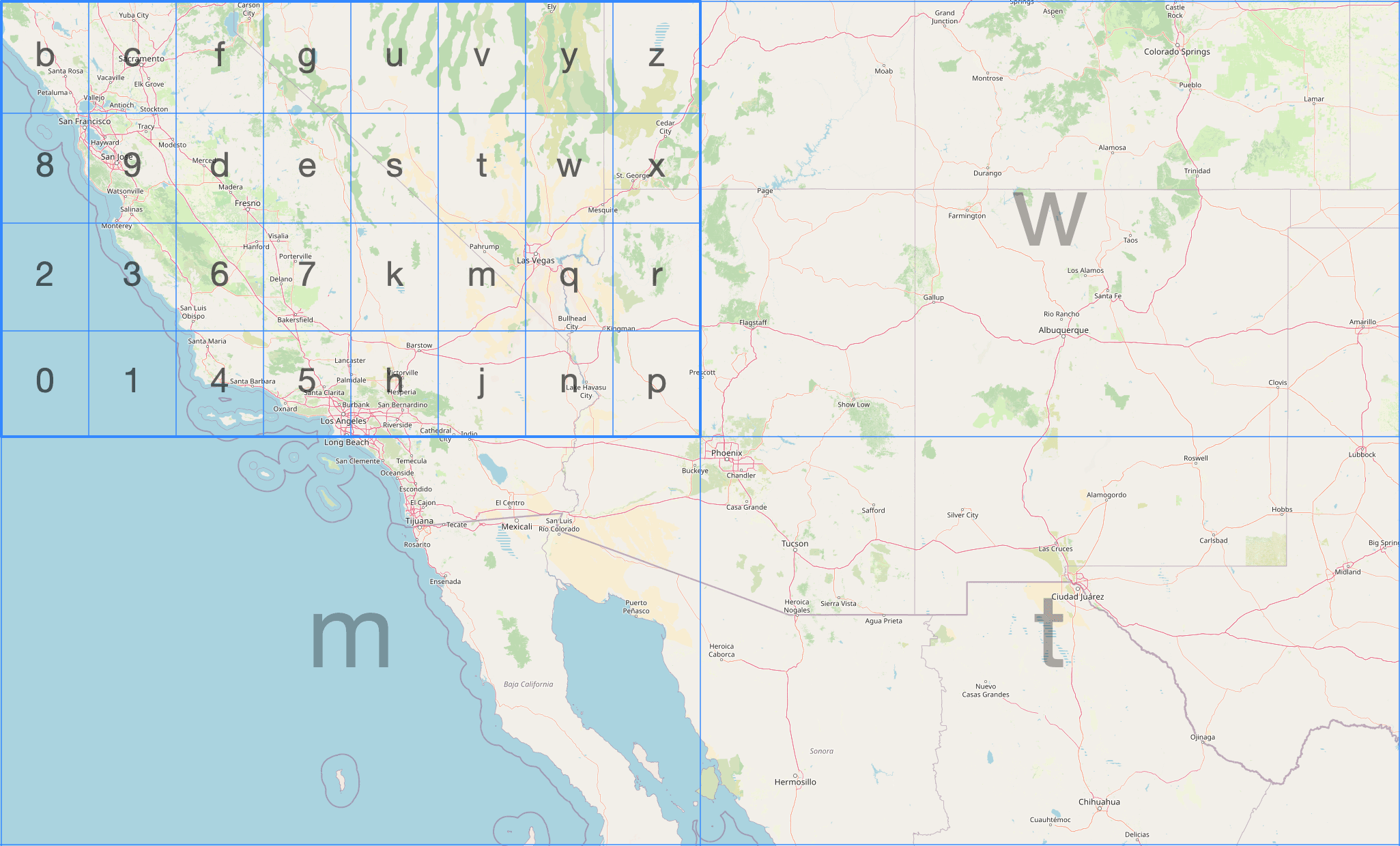
ClickHouse has three geohash functions. We can encode a point at a given precision (1–12) using geohashEncode:
1SELECT geohashEncode(-0.12, 51.5, 6);
┌─geohashEncode(-0.12, 51.5, 6)─┐
│ gcpuvr                        │
└───────────────────────────────┘
We can then decode back to the (longitude, latitude) of the cell center using the geoHashDecode function:
1SELECT geohashDecode('gcpuvr');
┌─geohashDecode('gcpuvr')──────────┐
│ {                               ↴│
│↳  "longitude": -0.1153564453125,↴│
│↳  "latitude": 51.50115966796875 ↴│
│↳}                                │
└──────────────────────────────────┘
We can also find all the geohash cells within a bounding box at a given precision using the geohashesInBox function:
1SELECT geohashesInBox(-0.5, 51.3, 0.3, 51.7, 4);
Row 1:
──────
geohashesInB⋯3, 51.7, 4): ['gcpe','gcps','gcpt','gcpw','gcpg','gcpu','gcpv','gcpy','u105','u10h','u10j','u10n']
Geohash cells are rectangles, not equal-area, and cells at the same level vary in size by latitude. It is simple and widely supported but not ideal for aggregations where you care about equal-area bucketing.
H3 #
H3 is Uber's hexagonal hierarchical indexing system. Hexagons tessellate without gaps, are roughly equal-area at a given resolution, and the hierarchy is clean - each cell has exactly 7 children at the next finer resolution (with a small number of pentagon exceptions).
The diagram below from the H3 docs shows the indexing system being applied to part of San Francisco:
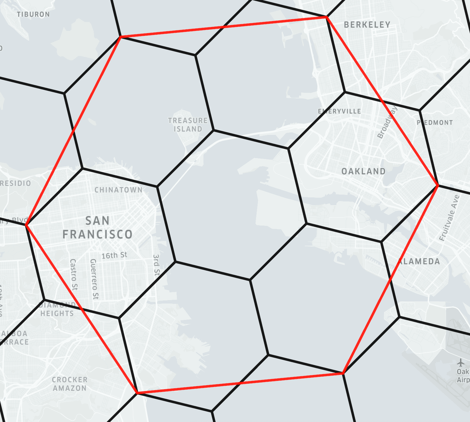
ClickHouse has 40+ H3 functions. We can encode a point to an H3 index at a given resolution using geoToH3. Note that unlike most ClickHouse geo functions, geoToH3 takes (latitude, longitude) order - matching H3's own convention:
1SELECT geoToH3(51.5, -0.12, 9);
┌─geoToH3(51.5, -0.12, 9)─┐
│      617438095026421759 │
└─────────────────────────┘
We can then decode back to the cell center using h3ToGeo:
1SELECT h3ToGeo(617438095026421759);
┌─h3ToGeo(617438095026421759)────────┐
│ {                                 ↴│
│↳  "latitude": 51.50008600604051,  ↴│
│↳  "longitude": -0.1214503427323559↴│
│↳}                                  │
└────────────────────────────────────┘
We can find the k-ring - the cell itself and all cells within k steps, using h3kRing:
1SELECT h3kRing(617438095026421759, 2);
Row 1:
──────
h3kRing(6174⋯6421759, 2): [617438095026421759,617438095026159615,617438095025111039,617438095025373183,617438095021441023,617438095022489599,617438095522922495,617438095522660351,617439388697624575,617438095026683903,617438095025635327,617438095025897471,617438095014100991,617438095013576703,617438095021703167,617438095020916735,617438095021965311,617438095522398207,617438095522136063]
We can find the parent cell at a coarser resolution using h3ToParent:
1SELECT h3ToParent(617438095026421759, 6);
┌─h3ToParent(6⋯6421759, 6)─┐
│       603927296197263359 │
└──────────────────────────┘
We can find the area of a cell in square meters using h3CellAreaM2:
1SELECT h3CellAreaM2(617438095026421759);
┌─h3CellAreaM2⋯5026421759)─┐
│         94179.9099582598 │
└──────────────────────────┘
We can find the grid distance between two cells using h3Distance:
1SELECT h3Distance(geoToH3(51.5, -0.12, 9), geoToH3(51.51, -0.11, 9));
┌─h3Distance(g⋯ -0.11, 9))─┐
│                        6 │
└──────────────────────────┘
H3 is excellent for aggregating observations by geography, computing catchment areas, and building hexagonal heatmaps. ClickHouse covers the full H3 API surface. We haven't covered all of them here - other useful ones include h3PolygonToCells (all cells covering a polygon), h3ToChildren (the inverse of h3ToParent), h3ToGeoBoundary (the polygon boundary of a cell, useful for visualization), and h3IsValid (validate a cell ID).
S2 #
S2 is Google's spherical geometry library. It starts by projecting the six faces of a cube onto the unit sphere, giving six top-level cells. Each cell is then subdivided into four children recursively, producing a hierarchy of quadrilateral cells at increasing levels of detail.
The image below, from the S2 docs, shows two of the six face cells, one of which has been subdivided several times:
S2 is used in Google Maps and BigQuery.
ClickHouse has 10+ S2 functions. We can encode a point to an S2 cell ID using geoToS2:
1SELECT geoToS2(-0.12, 51.5);
┌─geoToS2(-0.12, 51.5)─┐
│  5221366071371671575 │
└──────────────────────┘
We can decode back to the (longitude, latitude) of the cell center using s2ToGeo:
1SELECT s2ToGeo(5221366071371671575);
┌─s2ToGeo(5221366071371671575)──────────────┐
│ (-0.11999997687890043,51.499999963181374) │
└───────────────────────────────────────────┘
We can find the neighboring cells using s2GetNeighbors:
1SELECT s2GetNeighbors(5221366071371671575);
Row 1:
──────
s2GetNeighbo⋯1371671575): [5221366071371671613,5221366071371671577,5221366071371671569,5221366071371671573]
We can check whether two cells share any area using s2CellsIntersect:
1SELECT s2CellsIntersect(5221366071371671575, 5221366071371671613);
┌─s2CellsInter⋯1371671613)─┐
│                        0 │
└──────────────────────────┘
Adjacent cells share an edge but not area, so s2CellsIntersect returns 0.
For most use cases, H3 is the better choice. The main reason to reach for S2 is if your data comes from or needs to interoperate with BigQuery, which uses S2 natively via S2_CELLIDFROMPOINT and S2_COVERINGCELLIDS.
Which grid system to use? #
| Geohash | H3 | S2 | |
|---|---|---|---|
| Cell shape | Rectangle | Hexagon | Square (projected) |
| Equal area? | No | Approximately | Approximately |
| Hierarchy | Clean | Clean (×7) | Clean (×4) |
| ClickHouse support | 3 functions | 40+ functions | 10+ functions |
| Ecosystem | Very widely supported | Widely supported | Google ecosystem |
For new projects, H3 is usually the right choice. Geohash is good when you need interoperability with systems that already use it. S2 if you are working with BigQuery or Google Maps data.
Visualizing geometry #
svg() converts a geometry into an SVG element fragment - a Point becomes a <circle>, a Polygon becomes a <path>, a LineString becomes a <polygon>. Here we call it on a simplified London boundary polygon and the Tower of London point:
1SELECT 'london' AS name, svg(readWKT('POLYGON((-0.51 51.63,-0.10 51.69,0.26 51.65,0.33 51.52,0.25 51.30,-0.06 51.28,-0.33 51.32,-0.51 51.45,-0.51 51.63))')) AS fragment
2UNION ALL
3SELECT 'tower_of_london' AS name, svg((-0.0759, 51.5081)) AS fragment;
Row 1:
──────
name:     london
fragment: <g fill-rule="evenodd"><path d="M -0.51,51.63 L -0.1,51.69 L 0.26,51.65 L 0.33,51.52 L 0.25,51.3 L -0.06,51.28 L -0.33,51.32 L -0.51,51.45 L -0.51,51.63 z " style=""/></g>

Row 2:
──────
name:     tower_of_london
fragment: <circle cx="-0.0759" cy="51.5081" r="5" style=""/>
To build a viewable SVG, we can wrap the fragments in an <svg> tag with a viewBox covering our coordinate range. There are two things to handle:
- SVG's Y-axis points downward while latitude increases northward. We can fix this with a
scale(1,-1)transform. svg()uses a hardcodedr="5"for circles which is enormous relative to a geographic viewport. We can fix this using thereplaceOnefunction.
We end up with the following query, which also colors the point dark so that it's easier to see:
WITH
    readWKT('POLYGON((-0.51 51.63,-0.10 51.69,0.26 51.65,0.33 51.52,0.25 51.30,-0.06 51.28,-0.33 51.32,-0.51 51.45,-0.51 51.63))') AS london,
    (-0.0759, 51.5081) AS tower_of_london,
    replaceOne(svg(london), 'style=""', 'style="fill:#FAFF69;stroke:#1A1A2E;stroke-width:0.005"') AS london_svg,
    replaceOne(replaceOne(svg(tower_of_london), 'r="5"', 'r="0.02"'), 'style=""', 'style="fill:#161517;"') AS tower_svg
SELECT concat(
    '<svg xmlns="http://www.w3.org/2000/svg" viewBox="-0.55 51.24 0.92 0.49" width="600" height="300">',
    '<g transform="scale(1,-1) translate(0,-102.97)">',
    london_svg,
    tower_svg,
    '</g></svg>');
The output of this query is shown below:
<svg xmlns="http://www.w3.org/2000/svg" viewBox="-0.55 51.24 0.92 0.49" width="600" height="300"><g transform="scale(1,-1) translate(0,-102.97)"><g fill-rule="evenodd"><path d="M -0.51,51.63 L -0.1,51.69 L 0.26,51.65 L 0.33,51.52 L 0.25,51.3 L -0.06,51.28 L -0.33,51.32 L -0.51,51.45 L -0.51,51.63 z " style="fill:#FAFF69;stroke:#1A1A2E;stroke-width:0.005"/></g><circle cx="-0.0759" cy="51.5081" r="0.02" style="fill:#161517;"/></g></svg>
If we want to generate an SVG file and open it in a browser, we can run the following command:
clickhouse --query "
  WITH
      readWKT('POLYGON((-0.51 51.63,-0.10 51.69,0.26 51.65,0.33 51.52,0.25 51.30,-0.06 51.28,-0.33 51.32,-0.51 51.45,-0.51 51.63))') AS
  london,
      (-0.0759, 51.5081) AS tower_of_london,
      replaceOne(svg(london), 'style=\"\"', 'style=\"fill:#FAFF69;stroke:#1A1A2E;stroke-width:0.005\"') AS london_svg,
      replaceOne(replaceOne(svg(tower_of_london), 'r=\"5\"', 'r=\"0.02\"'), 'style=\"\"', 'style=\"fill:#161517;\"') AS tower_svg
  SELECT concat(
      '<svg xmlns=\"http://www.w3.org/2000/svg\" viewBox=\"-0.55 51.24 0.92 0.49\" width=\"600\" height=\"300\">',
      '<g transform=\"scale(1,-1) translate(0,-102.97)\">',
      london_svg,
      tower_svg,
      '</g></svg>')" > output.svg && open output.svg
The resulting SVG is shown below:

Spatial analytics in practice: NYC Taxis #
To make this concrete, let's use the NYC Taxi sample dataset with approximately 10 million trips, each with pickup and dropoff coordinates. We'll build an H3-indexed table, generate a hexagonal heatmap, identify the busiest pickup hotspots, and run a radius query — showing how the concepts from the previous sections fit together in practice.
First, the base table ordered first by pickup_datetime, which is its normal sort order:
1CREATE TABLE trips_small (
2    trip_id             UInt32,
3    pickup_datetime     DateTime,
4    dropoff_datetime    DateTime,
5    pickup_longitude    Nullable(Float64),
6    pickup_latitude     Nullable(Float64),
7    dropoff_longitude   Nullable(Float64),
8    dropoff_latitude    Nullable(Float64),
9    passenger_count     UInt8,
10    trip_distance       Float32,
11    fare_amount         Float32,
12    extra               Float32,
13    tip_amount          Float32,
14    tolls_amount        Float32,
15    total_amount        Float32,
16    payment_type        Enum('CSH' = 1, 'CRE' = 2, 'NOC' = 3, 'DIS' = 4, 'UNK' = 5),
17    pickup_ntaname      LowCardinality(String),
18    dropoff_ntaname     LowCardinality(String)
19) ENGINE = MergeTree
20ORDER BY (pickup_datetime, dropoff_datetime);
Let's insert the data:
1INSERT INTO trips_small
2SELECT * FROM s3(
3    'https://datasets-documentation.s3.eu-west-3.amazonaws.com/nyc-taxi/trips_{0..9}.gz',
4    'TabSeparatedWithNames'
5);
10000840 rows in set. Elapsed: 11.355 sec. Processed 10.00 million rows, 842.03 MB (880.76 thousand rows/s., 74.16 MB/s.)
Peak memory usage: 584.77 MiB.
We can confirm how many rows have been loaded by running the following query:
1SELECT count()
2FROM trips_small;
┌──count()─┐
│ 10000840 │ -- 10.00 million
└──────────┘
Now the H3 version. We add pickup_h3 and dropoff_h3 as MATERIALIZED columns - computed automatically at ingest from the coordinates - and put pickup_h3 first in the ORDER BY so spatial queries use the primary key index. Note the ifNull wrappers because the coordinate columns are Nullable:
1CREATE TABLE trips_small_h3 (
2    trip_id             UInt32,
3    pickup_datetime     DateTime,
4    dropoff_datetime    DateTime,
5    pickup_longitude    Nullable(Float64),
6    pickup_latitude     Nullable(Float64),
7    dropoff_longitude   Nullable(Float64),
8    dropoff_latitude    Nullable(Float64),
9    passenger_count     UInt8,
10    trip_distance       Float32,
11    fare_amount         Float32,
12    extra               Float32,
13    tip_amount          Float32,
14    tolls_amount        Float32,
15    total_amount        Float32,
16    payment_type        Enum('CSH' = 1, 'CRE' = 2, 'NOC' = 3, 'DIS' = 4, 'UNK' = 5),
17    pickup_ntaname      LowCardinality(String),
18    dropoff_ntaname     LowCardinality(String),
19    pickup_h3           UInt64 MATERIALIZED geoToH3(ifNull(pickup_latitude, 0), ifNull(pickup_longitude, 0), 9),
20    dropoff_h3          UInt64 MATERIALIZED geoToH3(ifNull(dropoff_latitude, 0), ifNull(dropoff_longitude, 0), 9)
21) ENGINE = MergeTree
22ORDER BY (pickup_h3, pickup_datetime);
Let's insert the data into this table, speeding things up by loading the data directly from trips_small instead of S3:
1INSERT INTO trips_small_h3
2SELECT *
3FROM trips_small;
10000840 rows in set. Elapsed: 9.766 sec. Processed 10.00 million rows, 723.35 MB (1.02 million rows/s., 74.06 MB/s.)
Peak memory usage: 424.98 MiB.
We can combine h3ToGeoBoundary with svg() to visualize the H3 grid directly from ClickHouse. h3ToGeoBoundary returns the cell boundary as a Ring in (latitude, longitude) order, so we swap coordinates with arrayMap before wrapping as a Polygon for svg(). We also need to flip the y-axis since SVG's y increases downward while latitude increases upward.
In the query below, we build a heatmap of the taxi trips with each H3 cell colored by log(trip count), and written to SVG format:
WITH cells AS (
    SELECT
        assumeNotNull(geoToH3(pickup_latitude, pickup_longitude, 9)) AS cell,
        count() AS trips
    FROM trips_small
    WHERE pickup_latitude BETWEEN 40.4 AND 40.95
      AND pickup_longitude BETWEEN -74.3 AND -73.7
    GROUP BY cell
    HAVING trips >= 10
),
max_trips AS (SELECT max(log(trips)) AS max_log FROM cells)
SELECT concat(
    '<svg xmlns="http://www.w3.org/2000/svg" viewBox="-74.05 40.58 0.32 0.35" width="650" height="1000" preserveAspectRatio="none">',
    '<rect x="-74.05" y="40.58" width="0.32" height="0.35" fill="#0a1628"/>',
    '<g transform="scale(1,-1) translate(0,-81.51)">',
    arrayStringConcat(groupArray(
        replaceAll(
            svg([arrayMap(p -> (p.2, p.1), h3ToGeoBoundary(cell))]::Polygon),
            'style=""',
            concat('style="fill:rgba(56,139,230,', toString(round(log(trips) / max_log, 3)), ');stroke:none"')
        )
    ), ''),
    '</g></svg>'
)
FROM cells, max_trips
FORMAT TSVRaw;
The FORMAT TSVRaw at the end outputs the raw string value with no table borders - without it, ClickHouse wraps the output in ┌─┐ characters that would break the SVG file.
Since the query contains single-quoted strings, save it to a file (e.g. h3_heatmap.sql) and run it with --queries-file. Pipe the output to an SVG file and open it in a browser:
1clickhouse --queries-file h3_heatmap.sql > h3_heatmap.svg

Manhattan is the bright diagonal strip running northeast to southwest - its grid is tilted ~29° from true north. Brooklyn spreads to the lower right, Queens to the right, and the two isolated bright clusters are LaGuardia (upper) and JFK (lower) airports.
We can now find the top pickup hotspots by grouping on the H3 cell:
1SELECT pickup_h3, count() AS trips
2FROM trips_small_h3
3WHERE pickup_h3 != 0
4GROUP BY pickup_h3
5ORDER BY trips DESC
6LIMIT 10;
┌──────────pickup_h3─┬──trips─┐
│ 617733123811311615 │ 168301 │
│ 619056821840379903 │ 136783 │
│ 617733123811835903 │ 122822 │
│ 617733124072407039 │  96570 │
│ 617733150971789311 │  92725 │
│ 617733123872391167 │  92066 │
│ 617733124388552703 │  90773 │
│ 617733123870818303 │  88238 │
│ 617733150972837887 │  83712 │
│ 617733123869507583 │  83588 │
└────────────────────┴────────┘

10 rows in set. Elapsed: 0.033 sec.
The second row - 136,783 trips at cell 619056821840379903 - is the bad-coordinate bucket we encountered earlier: those are the (0, 0) GPS failures that geoToH3 maps to a cell near the equator. We can filter it out by checking the cell center is within a plausible latitude range.
We can visualize these hotspots on the same heatmap we built above, highlighting the top 10 valid cells in white:
WITH all_cells AS (
      SELECT
          assumeNotNull(geoToH3(pickup_latitude, pickup_longitude, 9)) AS cell,
          count() AS trips
      FROM trips_small
      WHERE pickup_latitude BETWEEN 40.4 AND 40.95
        AND pickup_longitude BETWEEN -74.3 AND -73.7
      GROUP BY cell
      HAVING trips >= 10
  ),
  max_log AS (SELECT max(log(trips)) AS max_log FROM all_cells),
  top_cells AS (
      SELECT pickup_h3 AS cell, count() AS trips
      FROM trips_small_h3
      WHERE pickup_h3 != 0
      GROUP BY cell
      HAVING h3ToGeo(cell).latitude BETWEEN 40.0 AND 42.0
      ORDER BY trips DESC
      LIMIT 10
  ),
  background AS (
      SELECT replaceAll(
          svg([arrayMap(p -> (p.2, p.1), h3ToGeoBoundary(cell))]::Polygon),
          'style=""',
          concat('style="fill:rgba(250,255,105,', toString(round(log(trips) / max_log, 3)), ');stroke:none"')
      ) AS fragment
      FROM all_cells, max_log
  ),
  highlights AS (
      SELECT replaceAll(
          svg([arrayMap(p -> (p.2, p.1), h3ToGeoBoundary(cell))]::Polygon),
          'style=""',
          'style="fill:rgba(255,255,255,0.9);stroke:#161517;stroke-width:0.0005"'
      ) AS fragment
      FROM top_cells
  )
  SELECT concat(
      '<svg xmlns="http://www.w3.org/2000/svg" viewBox="-74.05 40.58 0.32 0.35" width="650" height="1000" preserveAspectRatio="none">',
      '<rect x="-74.05" y="40.58" width="0.32" height="0.35" fill="#161517"/>',
      '<g transform="scale(1,-1) translate(0,-81.51)">',
      arrayStringConcat((SELECT groupArray(fragment) FROM background), ''),
      arrayStringConcat((SELECT groupArray(fragment) FROM highlights), ''),
      '</g></svg>'
  )
  FORMAT TSVRaw;
Save to a file and pipe to SVG as before:
clickhouse --queries-file h3_hotspots.sql > h3_hotspots.svg

The white cells in the left cluster are all in Midtown Manhattan - the blocks around Penn Station, Grand Central, and Times Square. The two isolated white cells to the right are at LaGuardia Airport.
For a radius query - all pickups within two H3 cells of Times Square - h3kRing gives us the set of cells to look up, and the primary key index does the rest:
1SELECT count() AS trips
2FROM trips_small_h3
3WHERE pickup_h3 IN (
4    SELECT arrayJoin(h3kRing(geoToH3(40.758, -73.985, 9), 2))
5);
┌───trips─┐
│ 1144573 │ -- 1.14 million
└─────────┘

1 row in set. Elapsed: 0.006 sec.
The equivalent query against the base table uses a bounding box as there's no H3 index to lean on:
1SELECT count() AS trips
2FROM trips_small
3WHERE pickup_latitude BETWEEN 40.7525 AND 40.7633
4AND pickup_longitude BETWEEN -73.9925 AND -73.97
┌──trips─┐
│ 951983 │
└────────┘

1 row in set. Elapsed: 0.074 sec.
The H3 version is around 12 times faster on 10 million rows - a gap that widens significantly as data volume grows. The result counts differ because the bounding box is rectangular while the H3 k-ring is hexagonal - they cover a similar area with different shapes - the bounding box misses some trips in the corners of the outermost hexagonal cells.
When to use ClickHouse for geospatial in March 2026 #
ClickHouse excels at geospatial problems where the bottleneck is aggregate query speed on large datasets. If you're binning billions of location observations into H3 or geohash cells, running distance calculations or radius queries at scale, building hexagonal heatmaps, or enriching points with a fixed polygon boundary set via polygon dictionaries, ClickHouse is an excellent fit.
What ClickHouse doesn't do in geospatial in March 2026 #
ClickHouse doesn't support the full feature set of PostGIS, and for most analytical workloads that's fine as the performance advantage of what's supported is enormous. But, it's still worth knowing what's not currently supported.
No traditional spatial indexing. There is no R-tree index, but ClickHouse has effective alternatives. Storing H3 or geohash values in the primary key - as shown in the NYC taxi example above - is a form of spatial indexing: range scans on the primary key efficiently resolve spatial queries. quadtreemortonEncode(x, y) provides Morton-encoded quadtree indexing for Cartesian coordinates. The trade-off is that these approaches require knowing your query patterns at table design time.
No coordinate reference system (CRS) awareness. ClickHouse treats all coordinates as numbers. There is no reprojection, no EPSG code support, no awareness of whether your data is in WGS-84 or Web Mercator. You are responsible for ensuring your data is in a consistent CRS before ingesting.
areaSpherical does not return meters. As described earlier in this blog post, the spherical functions work on a unit sphere, which is maybe not obvious at first glance.
No ad-hoc spatial joins at index speed. Joining a table of millions of points against a table of hundreds of polygons at query time requires a pointInPolygon call on every row combination. For the common case of enriching points with a fixed set of boundaries - boroughs, regions, zones - the polygon dictionary approach described above solves this with an indexed lookup. But for arbitrary spatial joins between two large tables at query time, there is no equivalent of a spatial index join.
Function naming. If you are coming from PostGIS or any OGC-compliant database, the function names are different. e.g. pointInPolygon not ST_Contains, wkt() not ST_AsText, readWKTPolygon not ST_GeomFromText.
If your workload requires CRS-aware reprojection, complex topology operations (snapping, validation, simplification), or ad-hoc spatial joins between two large dynamic tables at query time, you'll likely need PostGIS or a dedicated GIS tool instead.
Where things are heading #
The introduction of the Geometry variant type in 2025 was the most significant architectural change to ClickHouse's geospatial support in several years. It makes the type system genuinely composable - you can write functions that accept any geometry type, store mixed data naturally, and ingest from external sources without knowing the geometry type in advance. The recent work to make all geometry functions accept both Geometry and the individual sub-types continues to smooth out the rough edges.
For analytics at scale on location data, ClickHouse is already an excellent choice. The tooling is mature, the performance is hard to beat, and the 2025 type system improvements mean the ergonomics are considerably better than they were.


