Global weather data from flying airplanes

Recently, I read the blog post by Niklas Oberhuber showing that it is possible to derive weather data from airplane telemetry. Airplanes don't broadcast temperature or wind data, but it can be calculated on the fly from other parameters. I immediately decided to reproduce these calculations to show something beautiful!

ADS-B Massive Visualizer collects telemetry from airplanes, such as their position, altitude, speed, and heading. This data is saved in the ClickHouse database. The service provides access to custom reports on top of over 150 billion data points and counting, accumulating them in real time.

You can read more about the service in the previous blog post.

Sensors #

Aircraft have many air pressure sensors, named "pitot tubes", which measure how the aircraft moves through the air. Static air pressure will show the altitude, and dynamic air pressure will show the airspeed relative to the air. These pressure sensors are the most important for flying dynamics.

Aircraft also have various navigation systems, which can show the altitude, speed, and heading, relative to the Earth. These measurements are less important to how the aircraft flies, but more important to navigation.

If we compare the values of these measurements to each other, we can derive more data. For example, comparing the airspeed with geometric speed will show us the speed of the tailwind (or headwind). Comparing the altitude from the pressure sensors with the geometric altitude could give some information about the local pressure changes and, maybe, temperature. Finally, comparing the heading relative to the air with the geometric heading will give us information about the wind direction.

Visualizations #

Let's suppose we want to visualize the angle (0..360 degrees) on the map. How to do it? We can use the color circle! So, different angles will be shown as different hues of color. For this purpose, ClickHouse provides functions for conversions between color spaces: colorOKLCHToSRGB and colorSRGBToOKLCH.

The color space that most of the displays and graphic cards use is named sRGB, and contains three channels (Red, Green, and Blue) that are Gamma-corrected (they are non-linear to provide more resolution to darker colors, as they are easier to distinguish relatively to each other than the brighter colors).

There is another color space, named OKLCH. It contains three channels: Lightness, Chroma, and Hue. It is cylindrical, because the L and C channels range in the line (say, between 0 and 1; however, some of the values can be out of range of the display device), and the Hue channel is circular (represents an angle between 0 and 360). It is designed to be linear (which means, if we do a linear gradient in that color space, the gradient will look okay, hence the name) and intended to be perceptually uniform (which means, if you average between two colors in that space, the resulting color is also perceived as the average; if you fix the Lightness and Chroma and change the Hue, the result will be perceived as having the same brightness).

Let's map aircraft headings using this color space:

Pressure #

Let's filter data for airplanes at least at 10,000 feet and map the difference between the altitude and geometric_altitude for a certain day:

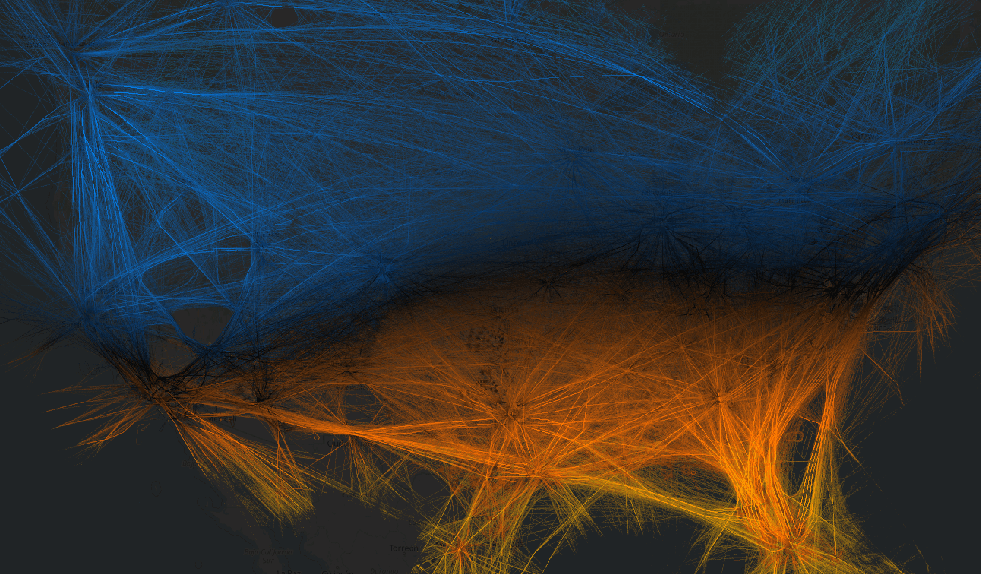
This looks surprisingly beautiful! Even more interesting, the picture changes if you select a different day.

I didn't derive the actual temperature from this data. The formula from Wikipedia looks complex, and I didn't want to apply it. Niklas Oberhuber also didn't use the formula but created a model instead. And I was just satisfied with nice pictures.

Crabbing angle #

When there is a strong but consistent crosswind, airplanes fly pointed into the wind. They can even land while pointed into the wind, which is called "crabbing". In the ADS-B data, there are two fields: one is track_degrees, which means the angle the plane points to, and another is aircraft_true_heading, which means the angle relative to the moving air around the airplane. If we subtract one angle from another, we will get the "crabbing" angle. Let's visualize it:

Unfortunately, most of the data is not available in the US, but it is available in the EU. Probably, it is due to some local regulations.

Wind #

Now let's calculate the wind direction and speed. It will require some trigonometry, and trying to understand these formulas is difficult without a pen and paper.

Here is the "crabbing angle" (or name it "drift angle") we calculated in the previous step:

positiveModulo(track_degrees - aircraft_true_heading + 180, 360) - 180 AS drift_angle,

The wind speed can be calculated in the following way: draw a triangle with the ground_speed as one side and the aircraft_tas (airspeed) as the other side, with the angle drift_angle between these two sides. The length of the other side (the difference between the vectors of ground_speed and aircraft_tas) is the wind speed:

sqrt(
    pow(ground_speed, 2) + pow(aircraft_tas, 2) -
    2 * ground_speed * aircraft_tas * cos(radians(drift_angle))
) AS wind_speed,

Use a similar rule to calculate the absolute wind direction angle:

positiveModulo(track_degrees +
    if(drift_angle < 0, -1, 1) * degrees(acos(
        greatest(-1, least(1,
            (pow(ground_speed, 2) + pow(wind_speed, 2) - pow(aircraft_tas, 2)) /
            (2 * ground_speed * if(wind_speed > 0.1, wind_speed, 1))
        ))
    )) + 180, 360
) AS wind_direction,

We would like to show the wind direction on the map. But sometimes one pixel on the map will contain multiple data points, and we need to aggregate them to calculate the average. How to calculate the average of angles, e.g., what is the average between 10 degrees and 350 degrees? (The answer should be zero.) Actually, we need even more: calculate the weighted average of wind direction angles with the wind speed as the weight, so the stronger wind will have a bigger contribution.

To do this, let's say that the wind direction and wind speed are polar coordinates of the wind vector. And what we need in the result is the average wind vector. The average is a function in the linear coordinate space, which is why we can't apply it simply in the polar coordinates. We can do a coordinate transform of the function, but put it more simply, we should convert our (direction, speed) coordinates to linear (x, y), then do the average across both x and y coordinates, then convert it back to the polar space and take the angle back as the average:

positiveModulo(degrees(atan2(
    avg(sin(radians(wind_direction)) * wind_speed),
    avg(cos(radians(wind_direction)) * wind_speed)
)), 360) AS avg_wind_direction,

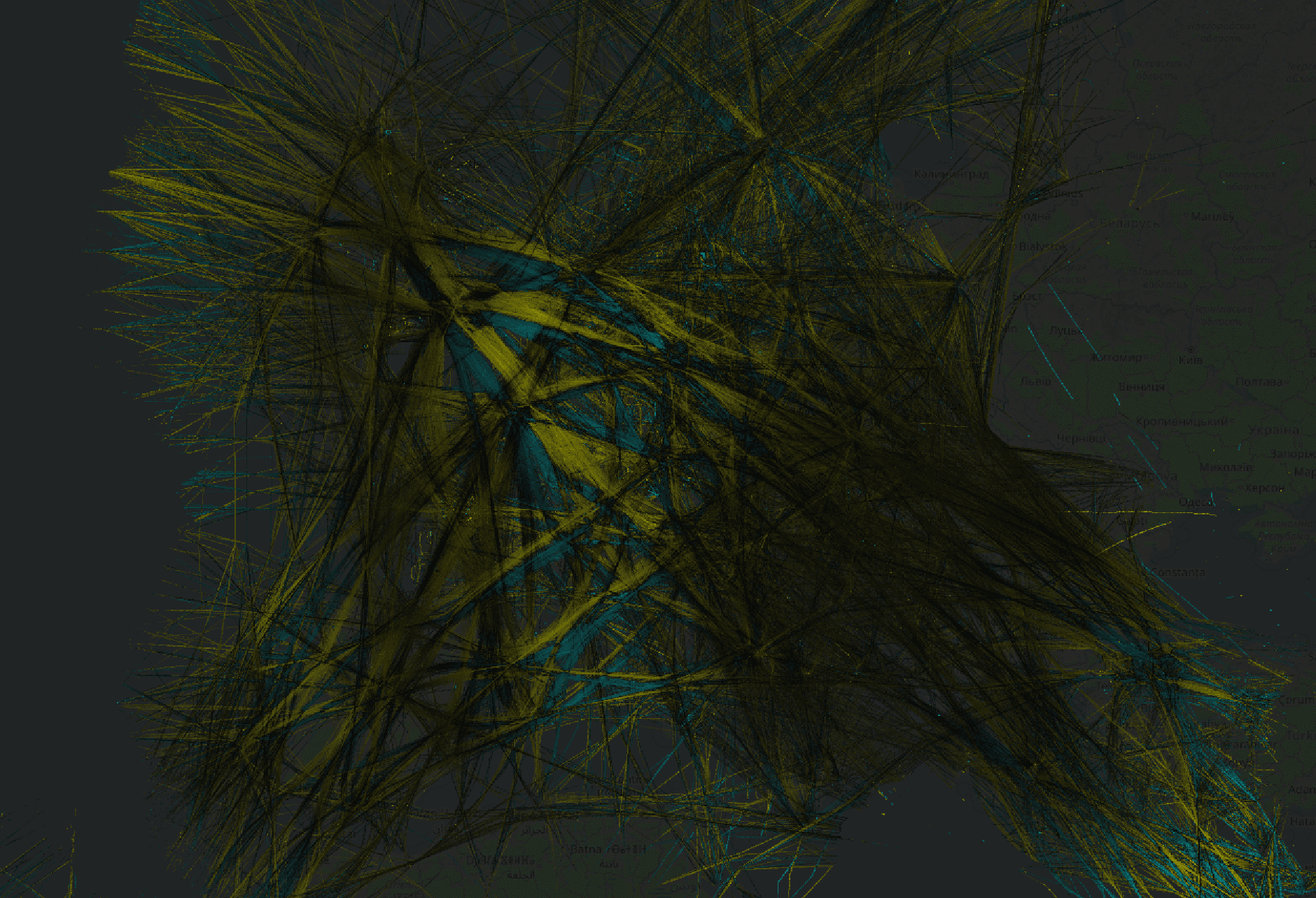
Now, given the wind angle and wind speed, it will be natural to map the angle to the color hue and the speed to the color lightness:

I compared the resulting picture to the actual weather data at https://earth.nullschool.net/ and it looked exactly as expected!

Bottom line #

ADS-B is a treasure trove of data, and it really shines when it is queryable in real-time with ClickHouse.

Bonus: how to do video visualizations. Prepare a query as follows. Copy it to adsb.exposed. Open the browser console. Copy and run the following snippet: frame = 0; const id = setInterval(() => { query_elem.value = query_elem.value.replace(/(\d+) AS frame/, ${frame} AS frame); updateMap(); if (frame >= 100) { clearInterval(id) }; ++frame; }, 10000). The first run is needed to bring the images to the cache. After it finishes, replace the update interval to one second, start recordmydesktop and repeat the run. The generated video can be processed with ffmpeg as follows: ffmpeg -y -i out.ogv -ss 4.5 -to 105 -filter:v "crop=2149:1218:893:666,thumbnail=15,setpts=0.1*PTS" -qscale:v 10 -an pressure.ogv, where the time offsets are found manually by looking at the video, and crop frame is determined by taking a screenshot and using the selection tool in the graphic editor. The ffmpeg invocation is constructed by Claude.