TL;DR
We added QBit to ClickHouse, a column type that stores floats as bit planes. It lets you choose how many bits to read during vector search, tuning recall and performance without changing the data.
Vector search is everywhere now. It powers music recommendations, retrieval-augmented generation (RAG) for large language models where external knowledge is fetched to improve answers, and even googling is powered by vector search to some extent. Many specialised databases are built to handle vector search very well. Nevertheless, these systems are rarely ideal for storing and querying structured data. As a result, we often see users preferring regular databases with ad-hoc vector capabilities over fully specialised vector stores.
In ClickHouse, brute-force vector search has been supported for several years already. More recently, we added methods for approximate nearest neighbour (ANN) search, including HNSW – the current standard for fast vector retrieval. We also revisited quantisation and built a new data type: QBit.
Each vector search method has its own parameters that decide trade-offs for recall, accuracy, and performance. Normally, these have to be chosen up-front. If you get them wrong, a lot of time and resources are wasted, and changing direction later becomes painful.
With QBit, no early decisions are needed. You can adjust precision and speed trade-off directly at query time, exploring the right balance as you go.
Vector search primer #
Let’s start with the basics. Vector search is used to find the most similar document (text, image, song, and so on) in a dataset. First, all items are converted into high-dimensional vectors (arrays of floats) using embedding models. These embeddings capture the meaning of the data. By comparing distances between vectors, we can see how close two items are in meaning.
Here’s a small example. Imagine we have embeddings for fruits and animals. Which one do you think sits closest to lemon? 🍋
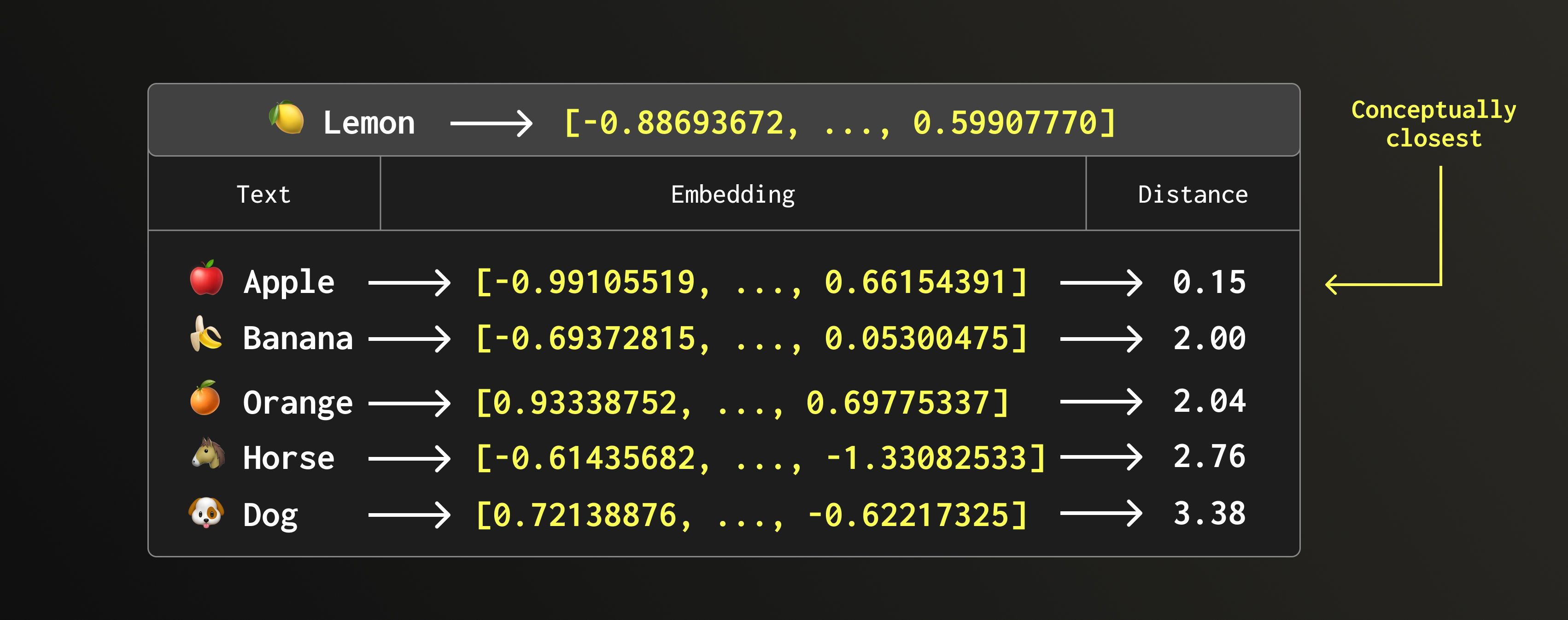
An apple! One might say this example is a bit silly. After all, lemon feels conceptually closer to orange or maybe banana because both are yellow. Still, this is a real example of brute-force search on rather small embeddings of size 5.
1CREATE TABLE fruit_animal
2ENGINE = MergeTree
3ORDER BY word
4AS SELECT *
5FROM VALUES(
6  'word String, vec Array(Float64)',
7  ('apple', [-0.99105519, 1.28887844, -0.43526649, -0.98520696, 0.66154391]),
8  ('banana', [-0.69372815, 0.25587061, -0.88226235, -2.54593015, 0.05300475]),
9  ('orange', [0.93338752, 2.06571317, -0.54612565, -1.51625717, 0.69775337]),
10  ('dog', [0.72138876, 1.55757105, 2.10953259, -0.33961248, -0.62217325]),
11  ('horse', [-0.61435682, 0.48542571, 1.21091247, -0.62530446, -1.33082533])
12);
1SELECT word, L2Distance(
2  vec, [-0.88693672, 1.31532824, -0.51182908, -0.99652702, 0.59907770]
3) AS distance
4FROM fruit_animal
5ORDER BY distance
6LIMIT 5;
   ┌─word───┬────────────distance─┐
1. │ apple  │ 0.14639757188169716 │
2. │ banana │  1.9989613690076786 │
3. │ orange │   2.039041552613732 │
4. │ horse  │  2.7555776805484813 │
5. │ dog    │   3.382295083120104 │
   └────────┴─────────────────────┘
Higher-dimensional embeddings can represent more complex relationships and produce richer results. But hopefully, we can all agree that horse and dog being at the bottom of the list feels about right.
Approximate Nearest Neighbours (ANN) #
Exact vector search is powerful but slow, and therefore costly. Many applications can tolerate a bit of flexibility. For example, it’s fine if, after listening to Eminem, you’re recommended Snoop Dogg or Tupac. But something has gone very wrong if the next suggestion is this.
That’s why Approximate Nearest Neighbour (ANN) techniques exist. They provide faster and cheaper retrievals at the expense of perfect accuracy. The two most common approaches are quantisation and HNSW.
We’ll look briefly at both, and then see how QBit fits into this picture.
Quantisation #
Suppose our stored vectors are of type Float64, and we’re not happy with the performance. The natural question is: what if we downcast the data to a smaller type?
Smaller numbers mean smaller data, and smaller data means faster distance calculations. ClickHouse’s vectorized query execution engine can fit more values into processor registers per operation, increasing throughput directly. On top of that, reading fewer bytes from disk reduces I/O load. This idea is known as quantisation.
When quantising, we have to decide how to store the data. We can either:
- Keep the quantised copy alongside the original column, or
- Replace the original values entirely (by downcasting on insertion).
The first option doubles storage, but it’s safe as we can always fall back to full precision. The second option saves space and I/O, but it’s a one-way door. If later we realise the quantisation was too aggressive and results are inaccurate, there’s no way back.
Hierarchical Navigable Small World (HNSW) #
There are many data structures designed to find the nearest neighbour without scanning all candidates. We call them indexes. Among them, HNSW is often seen as the monarch.
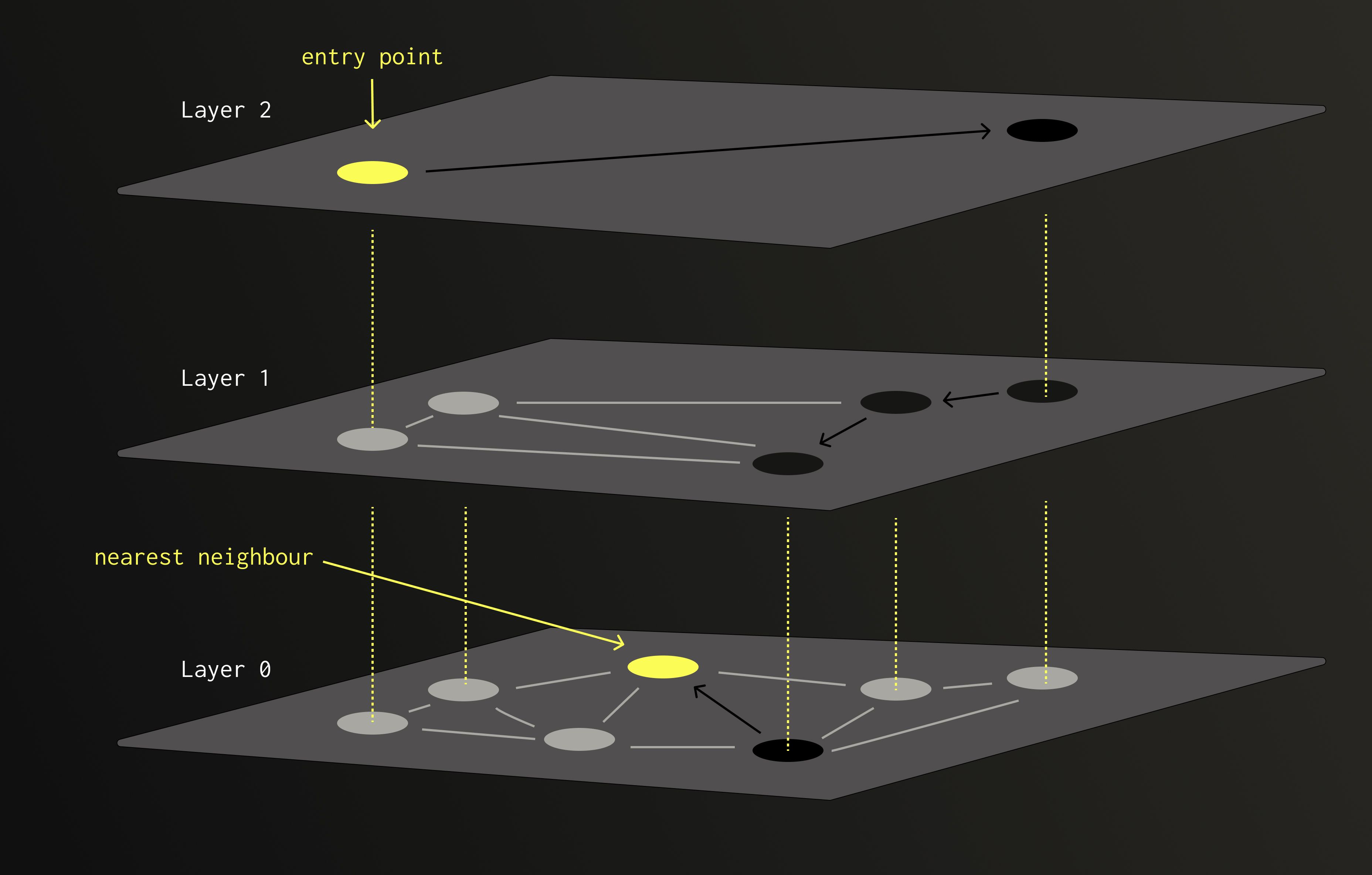
HNSW is built from multiple layers of nodes (vectors). Each node is randomly assigned to one or more layers, with the chance of appearing in higher layers decreasing exponentially.
When performing a search, we start from a node at the top layer and move greedily towards the closest neighbours. Once no closer node can be found, we descend to the next, denser layer, and continue the process. The higher layers provide long-range connections to avoid getting trapped in local minima, while the lower layers ensure precision.
Because of this layered design, HNSW achieves logarithmic search complexity with respect to the number of nodes. Far faster than the linear scans used in brute-force search or quantisation-based methods.
The main bottleneck is memory. ClickHouse uses the usearch implementation of HNSW, which is an in-memory data structure that doesn’t support splitting. As a result, larger datasets require proportionally more RAM. Quantising the data before building the index can help reduce this footprint, but many HNSW parameters still have to be chosen in advance, including the quantisation level itself. And this is exactly the rigidity that QBit set out to address.
Quantised Bit (QBit) #
QBit is a new data structure that can store BFloat16, Float32, and Float64 values by taking advantage of how floating-point numbers are represented – as bits. Instead of storing each number as a whole, QBit splits the values into bit planes: every first bit, every second bit, every third bit, and so on.
When running a search, ClickHouse can read just the required subcolumns to reconstruct the data up to the user-specified precision.

This approach solves the main limitation of traditional quantisation. There’s no need to store duplicated data or risk making values meaningless. It also avoids the RAM bottlenecks of HNSW, since QBit works directly with the stored data rather than maintaining an in-memory index.
Most importantly, no upfront decisions are required. Precision and performance can be adjusted dynamically at query time, allowing users to explore the balance between accuracy and speed with minimal friction.
Although QBit speeds up vector search, its computational complexity remains O(n). In other words: if your dataset is small enough for an HNSW index to fit comfortably in RAM, that is still the fastest choice.
| Category | Brute-force | HNSW | QBit |
|---|---|---|---|
| Precision | Perfect | Great | Flexible |
| Speed | Slow | Fast | Flexible |
| Others | Quantized: more space or irreversible precision | Index has to fit in memory and has to be built | Still O(#records) |
QBit deepdive #
Let’s revisit the familiar example, but this time, in the world of QBit.
1CREATE TABLE fruit_animal
2(
3    word String,
4    vec QBit(Float64, 5)
5)
6ENGINE = MergeTree
7ORDER BY word;
8
9INSERT INTO fruit_animal VALUES
10('apple',  [...]),
11('banana', [...]),
12('orange', [...]),
13('dog',    [...]),
14('horse',  [...]);
Now we can run a query:
1SELECT
2  word,
3  L2DistanceTransposed(vec, [...], 16) AS distance
4FROM fruit_animal
5ORDER BY distance;
   ┌─word───┬────────────distance─┐
1. │ apple  │ 0.14639757188169716 │
2. │ banana │   1.998961369007679 │
3. │ orange │   2.039041552613732 │
4. │ cat    │   2.752802631487914 │
5. │ horse  │  2.7555776805484813 │
6. │ dog    │   3.382295083120104 │
   └────────┴─────────────────────┘
Interactions with QBit can be split into two parts:
- The data type itself: its creation and data ingestion.
- Distance calculations.
Let’s look into both.
The data type #
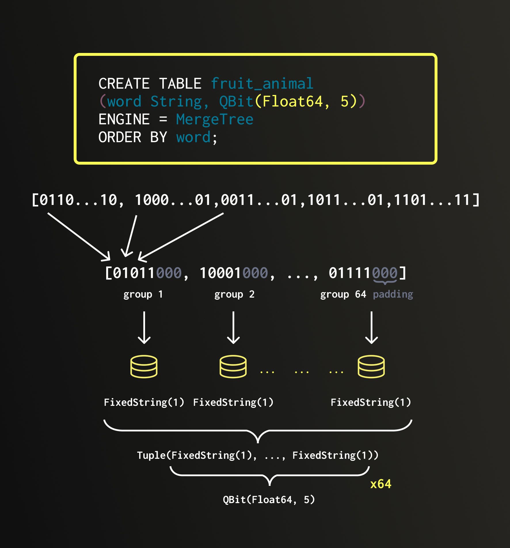
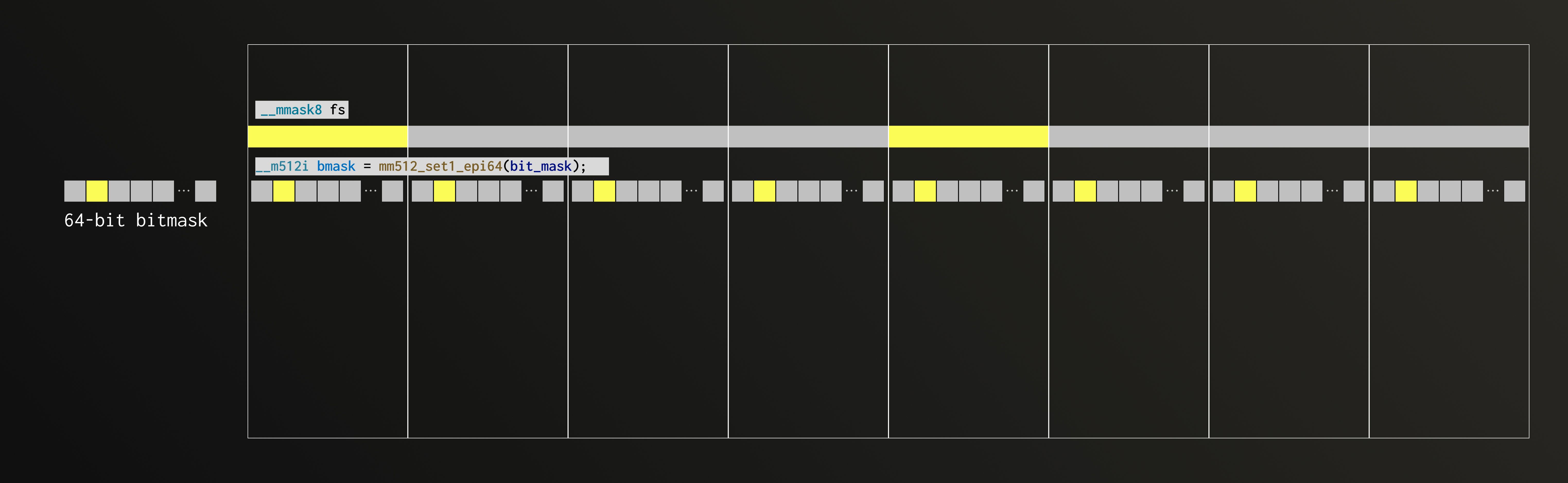
When data is inserted into a QBit column, it is transposed so that all first bits line up together, all second bits line up together, and so on. We call these groups.
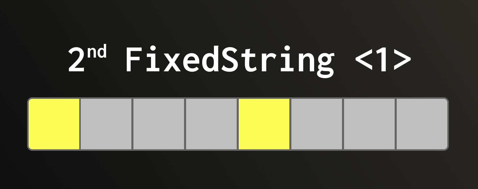
Each group is stored in a separate FixedString(N) column: fixed-length strings of N bytes stored consecutively in memory with no separators between them. All such groups are then bundled together into a single Tuple, which forms the underlying structure of QBit.
If we start with a vector of 8×Float64 elements, each group will contain 8 bits. Because a Float64 has 64 bits, we end up with 64 groups (one for each bit). Therefore, the internal layout of QBit(Float64, 8) looks like a Tuple of 64×FixedString(1) columns.
If the original vector length doesn’t divide evenly by 8, the structure is padded with invisible elements to make it align to 8. This ensures compatibility with FixedString, which operates strictly on full bytes. For example, in the picture above, the vector contains 5 Float64 values. It would be padded by three zeroes producing 8×Float64, which is then transposed into a Tuple of 64×FixedString(1). Or, if we started with 76×BFloat16 elements, we would pad it to 80×BFloat16 and transpose it into a Tuple of 16×FixedString(10).
The distance calculation #
1SELECT
2  word,
3  L2DistanceTransposed(vec, [...], 16) AS distance
4FROM fruit_animal
5ORDER BY distance;
I/O Optimisation #
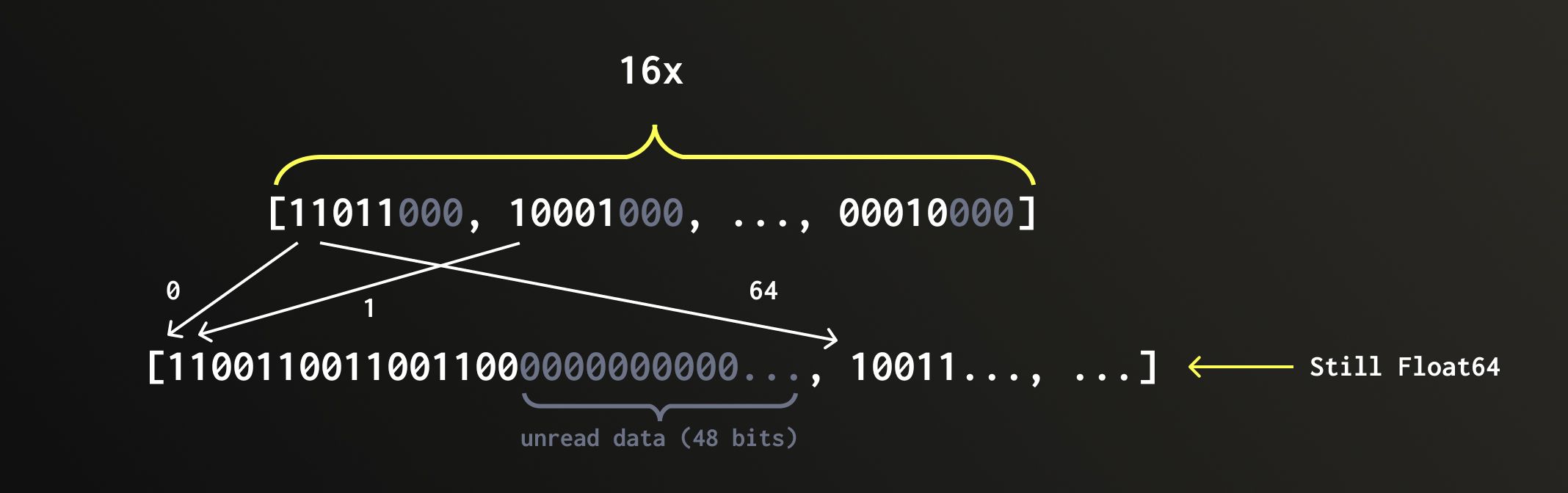
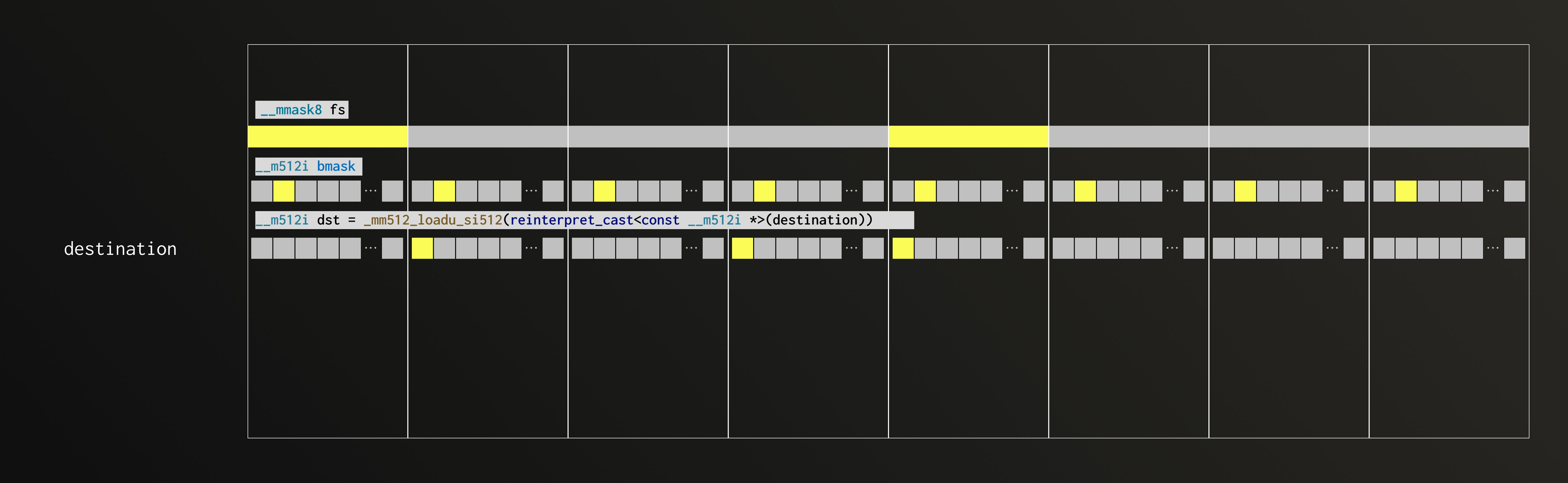
Before we can calculate distances, the required data must be read from disk and then untransposed (converted back from the grouped bit representation into full vectors). Because QBit stores values bit-transposed by precision level, ClickHouse can read only the top bit planes needed to reconstruct numbers up to the desired precision.
In the query above, we use a precision level of 16. Since a Float64 has 64 bits, we only read the first 16 bit planes, skipping 75% of the data.
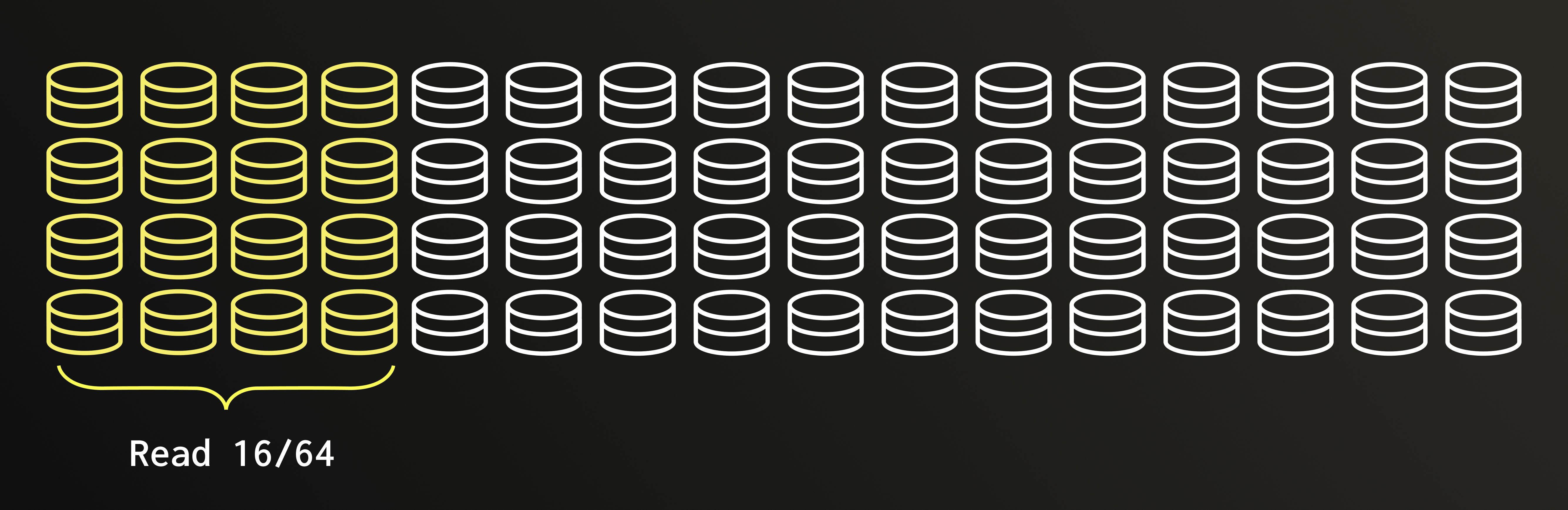
After reading, we reconstruct only the top portion of each number from the loaded bit planes, leaving the unread bits zeroed out.
Calculation optimisation #
One might ask whether casting to a smaller type, such as Float32 or BFloat16, could eliminate this unused portion. It does work, but explicit casts are expensive when applied to every row. Instead, we can downcast only the reference vector and treat the QBit data as if it contained narrower values (“forgetting” the existence of some columns), since its layout often corresponds to a truncated version of those types. But not always!
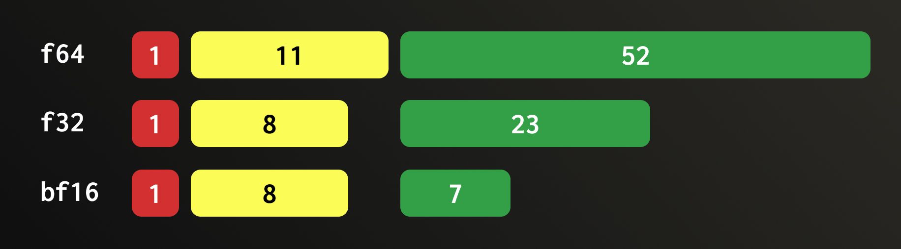
Let’s start with the simple case where the original data is Float32, and the chosen precision is 16 bits or fewer. BFloat16 is a Float32 truncated by half. It keeps the same sign bit and 8-bit exponent, but only the upper 7 bits of the 23-bit mantissa. Because of this, reading the first 16 bit planes from a QBit column effectively reproduces the layout of BFloat16 values. So in this case, we can (and do) safely convert the reference vector (the one all the data in QBit is compared against) to BFloat16 and treat the QBit data as if it were stored that way from the start.
Float64, however, is a different story. It uses an 11-bit exponent and a 52-bit mantissa, meaning it’s not simply a Float32 with twice the bits. Its structure and exponent bias are completely different. Downcasting a Float64 to a smaller format like Float32 requires an actual IEEE-754 conversion, where each value is rounded to the nearest representable Float32. This rounding step is computationally expensive and cannot be replaced with simple bit slicing or permutation.
The same holds when the precision is 16 or smaller. Converting from Float64 to BFloat16 is effectively the same as first converting to Float32 and then truncating that to BFloat16. So here too, bit-level tricks won’t help.
Let’s vectorise #
What’s vectorisation #
The main performance difference between regular quantised columns and QBit columns is the need to untranspose the bit-grouped data back into vector form during search. Doing this efficiently is critical. ClickHouse has a vectorized query execution engine, so it makes sense to use it to our advantage. You can read more about vectorisation in this ClickHouse blog post.
In short, vectorisation allows the CPU to process multiple values in a single instruction using SIMD (Single-Instruction-Multiple-Data) registers. The term originates from the fact that SIMD instructions operate on small batches (vectors) of data. Individual elements within these vectors are of fixed length and are typically referred to as lanes.
There are two common approaches to vectorising algorithms:
-
Auto-vectorisation. Write an algorithm in such a way that the compiler will figure out the concrete SIMD instructions itself. As compilers can only do this with very simple straight-forward functions, usually such a way is only achievable if the architecture of your system is carefully designed around an auto-vectorising algorithm, like here.
-
Intrinsics. Write the algorithm using explicit intrinsics: special functions that compilers map directly into CPU instructions. These are platform dependent, but offer full control.
General algorithm #
SIMD untransposition is too complex for the compiler to auto-vectorise, so we’ve taken the second route and will walk you through it. Let’s first look at the idea behind the algorithm, and then see how it fits into the vectorized world.
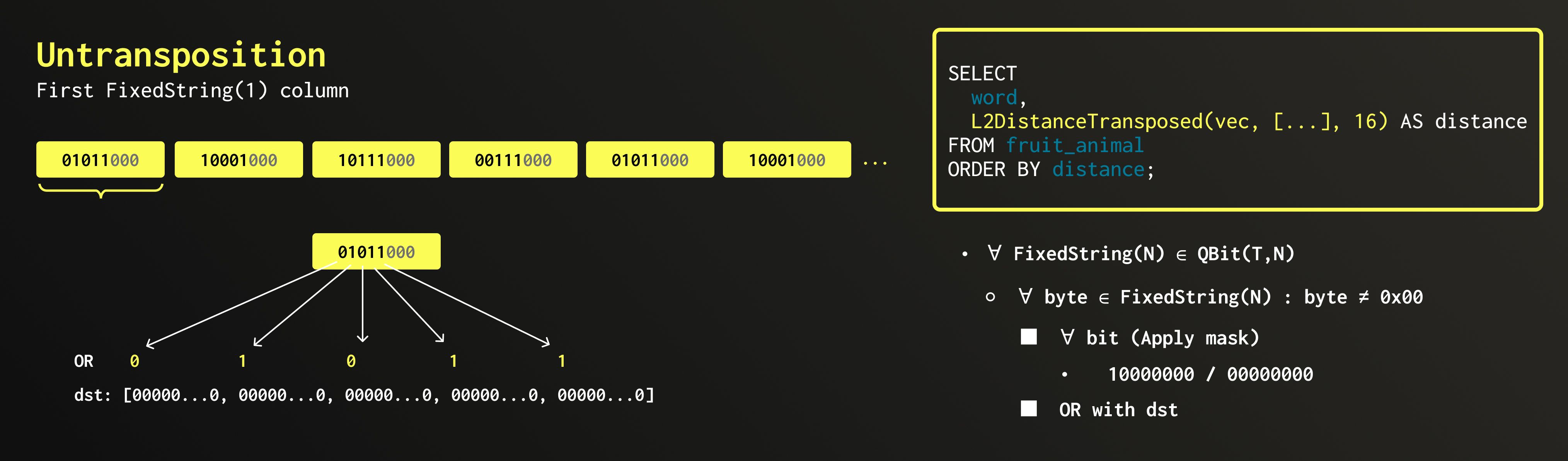
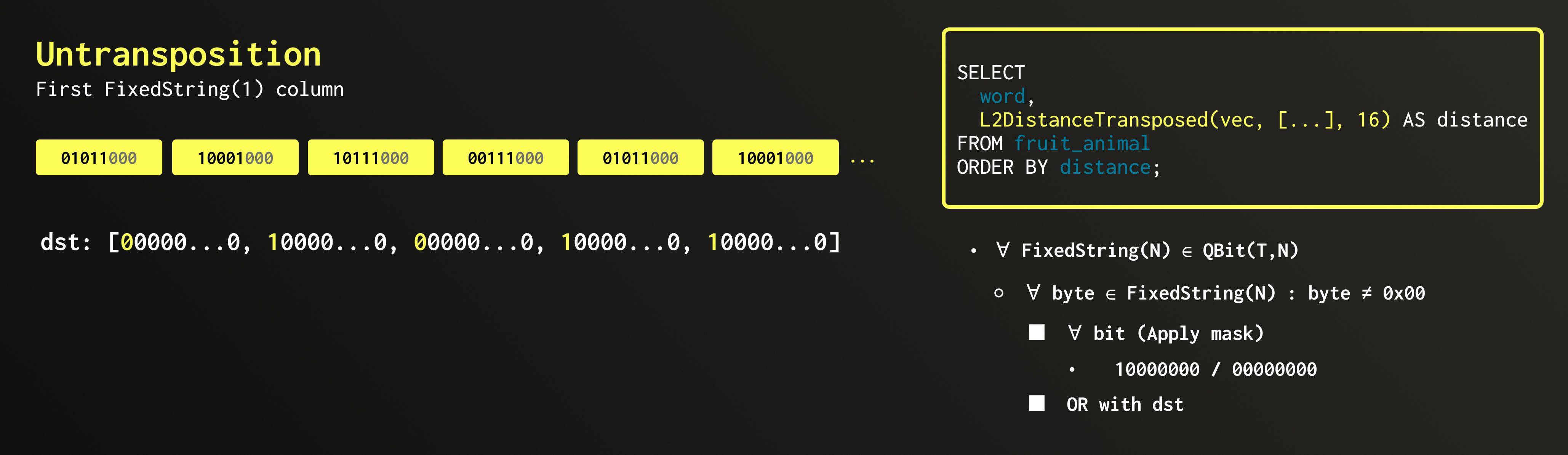
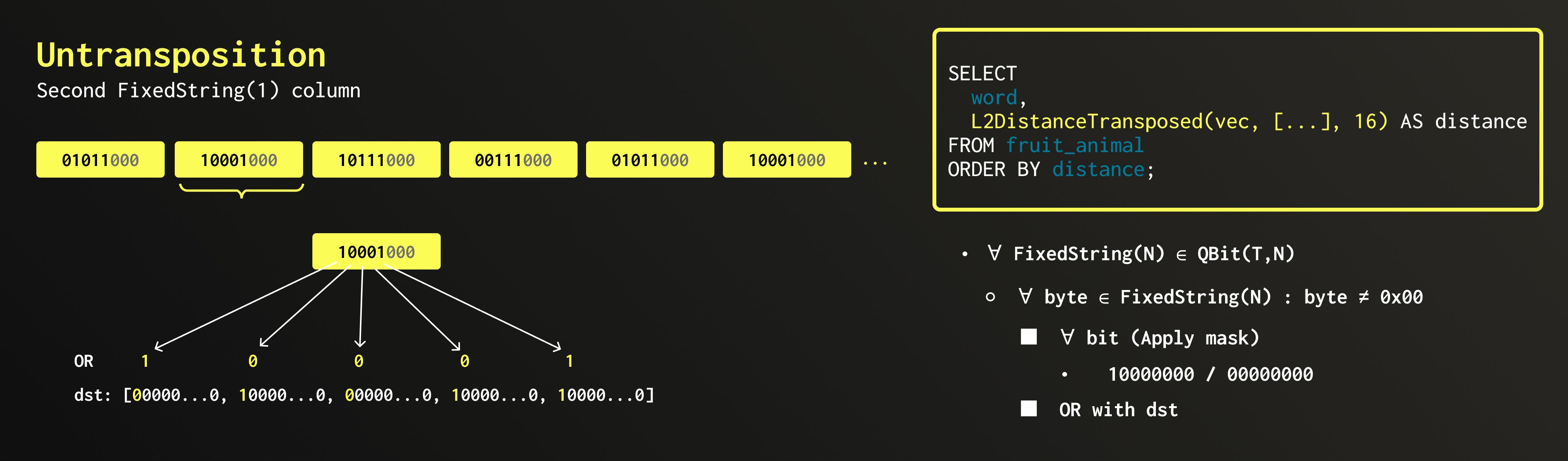
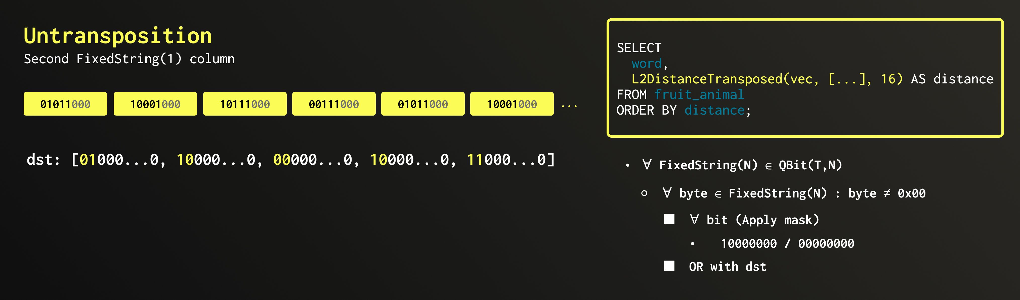
We loop through all FixedString columns of the QBit (64 of them for Float64). Within each column, we iterate over every byte of the FixedString, and within each byte, over every bit.
If a bit is 0, we apply a zero mask to the destination at the corresponding position. If a bit is 1, we apply a mask that depends on its position within the byte. For example, if we are processing the first bit, the mask is 10000000; for the second bit, it becomes 01000000, and so on. The operation we apply is a logical OR, merging the bit from the source into the destination byte.
Vectorized algorithm #
Let’s now look at the second iteration (steps 3 and 4 from above) using AVX-512, an instruction set that’s common across modern CPUs. In this example, we’re unpacking the second FixedString(1) group and each bit here contributes to the second bit of eight resulting Float64 values.
When dealing with SIMD, it’s easier to think in lanes. AVX-512 operates on 512-bit registers, which correspond to eight 64-bit lanes. Let’s map our fixed strings across those lanes to visualise the data layout.
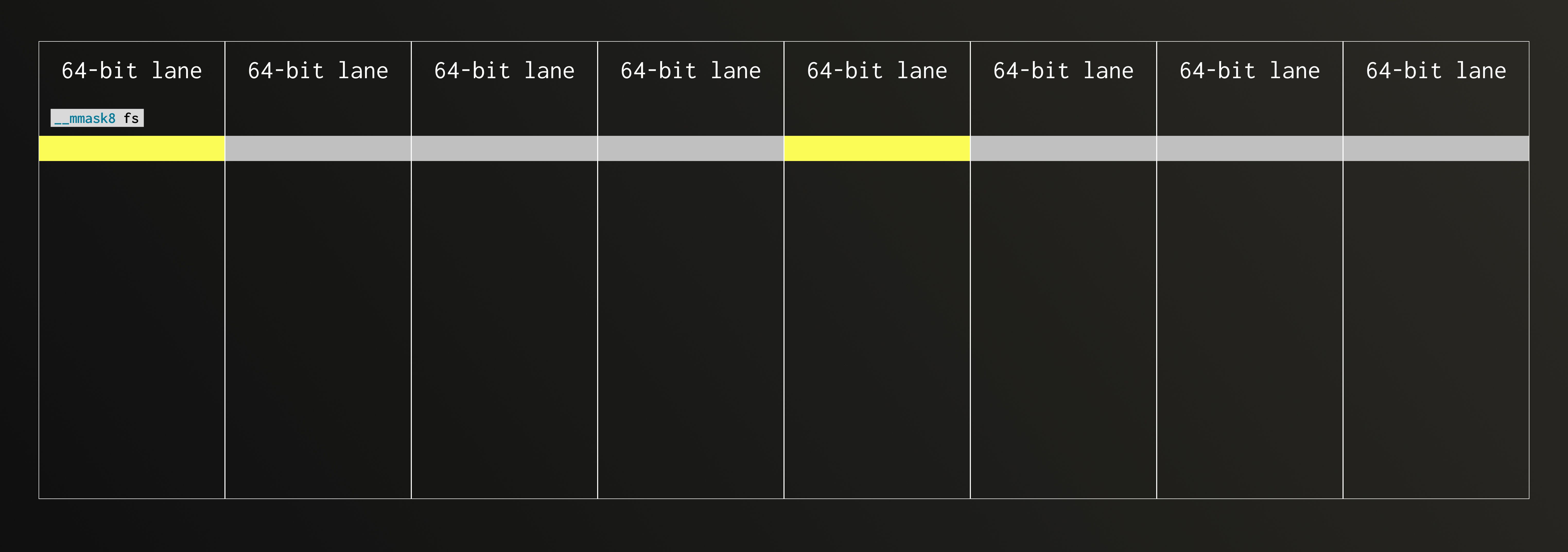
Since we’re unpacking the second bit of each Float64, the bitmask now has its second bit set.
We apply that mask across the lanes.
The destination (dst) already contains results from the previous iteration. We are working on merging in the second bit as well.
Now comes the interesting part. If our mask were all ones, we’d simply OR the new bits into the destination (this case is what we call upd). If the mask were all zeros, the destination would stay unchanged. In practice, each bit of the mask decides which lane to update: where the mask is 1, take the value from upd; where it’s 0, keep the old one. Luckily, AVX-512 provides an intrinsic that does exactly this: it merges elements conditionally within the lanes, choosing between upd and the dst based on the mask bits.
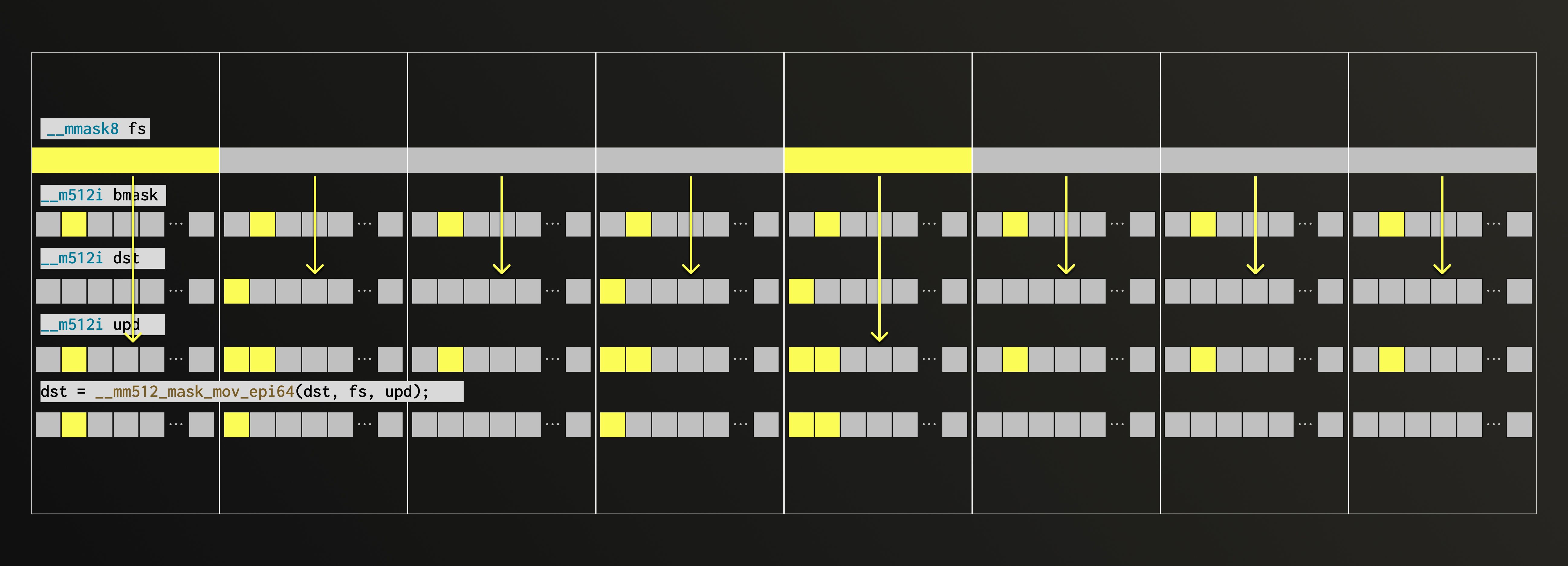
Congratulations, we’ve just unpacked eight values in a single iteration!
Now that the data is ready, we can compute distances. For that, we use SimSimd, an amazing library that performs vectorized distance calculations on almost any hardware.
Benchmarks #
We ran benchmarks on the HackerNews dataset, which contains around 29 million comments represented as Float32 embeddings. We measured the speed of searching for a single new comment (using its embedding) and computed the recall based on 10 new comments.
Recall here is the fraction of true nearest neighbours that appear among the top-k retrieved results (in our case, k = 20). Granularity is how many bit groups we read.
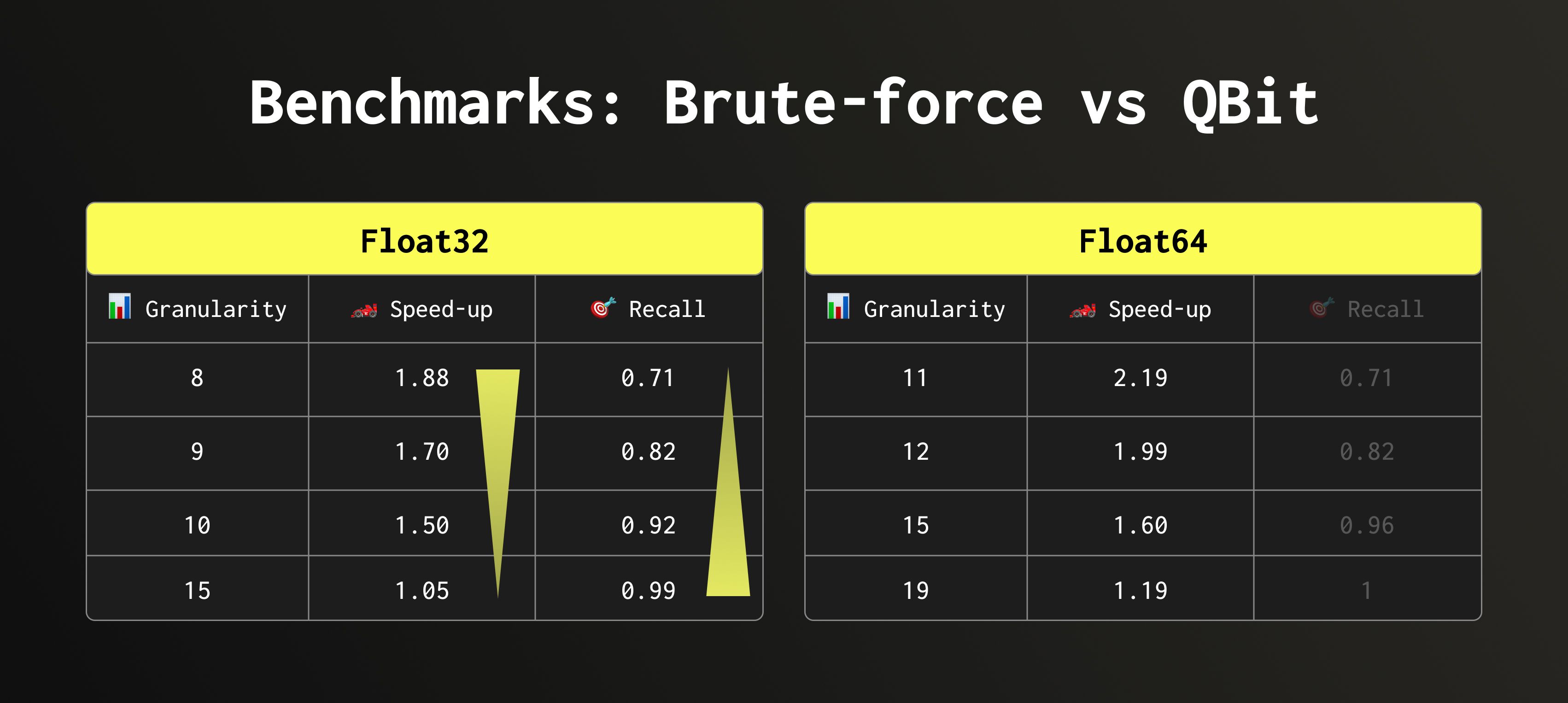
We achieved nearly 2× speed-up with a good recall. More importantly, we can now control the speed-accuracy balance directly, adjusting it to match the workload.
Take the Float64 recall results with a grain of salt: these embeddings are simply upcast versions of Float32, so the lower half of the Float64 bits carries little to none information, thus removing them didn’t affect the recall as much as it can. Speed-up values, however, are fully reliable in both cases.
But benchmarks are boring. Let’s have some fun!
Fun #
Create a table and download the data for DBpedia. It contains 1 million Wikipedia articles represented as Float32 embeddings. Now, add a QBit column:
1set allow_experimental_qbit_type = 1;
2ALTER TABLE dbpedia ADD COLUMN qbit QBit(Float32, 1536);
3ALTER TABLE dbpedia UPDATE qbit = vector WHERE 1;
Let’s start with a brute-force search. We’ll look for concepts most related to all space-related search terms: Moon, Apollo 11, Space Shuttle, Astronaut, Rocket. Or, if we want to be technical:
Search the top 1000 semantically similar entries to each of the five concepts. Return entries that appear in at least three of those results, ranked by how many concepts they match and their minimum distance to any of them (excluding the originals).
The full query is available on Pastila as it’s long. Here are the results:
Row 1:
──────
title:                Apollo program
text:                 The Apollo program, also known as Project Apollo, was the third United States human spaceflight program carried out by the National Aeronautics and Space Administration (NASA), which accomplished landing the first humans on the Moon from 1969 to 1972. First conceived during Dwight D. Eisenhower's administration as a three-man spacecraft to follow the one-man Project Mercury which put the first Americans in space, Apollo was later dedicated to President John F.
num_concepts_matched: 4
min_distance:         0.82420665
avg_distance:         1.0207901149988174

Row 2:
──────
title:                Apollo 8
text:                 Apollo 8, the second human spaceflight mission in the United States Apollo space program, was launched on December 21, 1968, and became the first manned spacecraft to leave Earth orbit, reach the Earth's Moon, orbit it and return safely to Earth.
num_concepts_matched: 4
min_distance:         0.8285278
avg_distance:         1.0357224345207214

Row 3:
──────
title:                Lunar Orbiter 1
text:                 The Lunar Orbiter 1 robotic (unmanned) spacecraft, part of the Lunar Orbiter Program, was the first American spacecraft to orbit the Moon.  It was designed primarily to photograph smooth areas of the lunar surface for selection and verification of safe landing sites for the Surveyor and Apollo missions. It was also equipped to collect selenodetic, radiation intensity, and micrometeoroid impact data.The spacecraft was placed in an Earth parking orbit on August 10, 1966 at 19:31 (UTC).
num_concepts_matched: 4
min_distance:         0.94581836
avg_distance:         1.0584313124418259

Row 4:
──────
title:                Apollo (spacecraft)
text:                 The Apollo spacecraft was composed of three parts designed to accomplish the American Apollo program's goal of landing astronauts on the Moon by the end of the 1960s and returning them safely to Earth.  The expendable (single-use) spacecraft consisted of a combined Command/Service Module (CSM) and a Lunar Module (LM).
num_concepts_matched: 4
min_distance:         0.9643517
avg_distance:         1.0367188602685928

Row 5:
──────
title:                Surveyor 1
text:                 Surveyor 1 was the first lunar soft-lander in the unmanned  Surveyor program of the National Aeronautics and Space Administration (NASA, United States). This lunar soft-lander gathered data about the lunar surface that would be needed for the manned Apollo Moon landings that began in 1969.
num_concepts_matched: 4
min_distance:         0.9738264
avg_distance:         1.0988530814647675

Row 6:
──────
title:                Spaceflight
text:                 Spaceflight (also written space flight) is ballistic flight into or through outer space. Spaceflight can occur with spacecraft with or without humans on board. Examples of human spaceflight include the Russian Soyuz program, the U.S. Space shuttle program, as well as the ongoing International Space Station. Examples of unmanned spaceflight include space probes that leave Earth orbit, as well as satellites in orbit around Earth, such as communications satellites.
num_concepts_matched: 4
min_distance:         0.9831049
avg_distance:         1.060678943991661

Row 7:
──────
title:                Skylab
text:                 Skylab was a space station launched and operated by NASA and was the United States' first space station. Skylab orbited the Earth from 1973 to 1979, and included a workshop, a solar observatory, and other systems. It was launched unmanned by a modified Saturn V rocket, with a weight of 169,950 pounds (77 t).  Three manned missions to the station, conducted between 1973 and 1974 using the Apollo Command/Service Module (CSM) atop the smaller Saturn IB, each delivered a three-astronaut crew.
num_concepts_matched: 4
min_distance:         0.99155205
avg_distance:         1.0769911855459213

Row 8:
──────
title:                Orbital spaceflight
text:                 An orbital spaceflight (or orbital flight) is a spaceflight in which a spacecraft is placed on a trajectory where it could remain in space for at least one orbit. To do this around the Earth, it must be on a free trajectory which has an altitude at perigee (altitude at closest approach) above 100 kilometers (62 mi) (this is, by at least one convention, the boundary of space).  To remain in orbit at this altitude requires an orbital speed of ~7.8 km/s.
num_concepts_matched: 4
min_distance:         1.0075209
avg_distance:         1.085978478193283

Row 9:
───────
title:                Dragon (spacecraft)
text:                 Dragon is a partially reusable spacecraft developed by SpaceX, an American private space transportation company based in Hawthorne, California. Dragon is launched into space by the SpaceX Falcon 9 two-stage-to-orbit launch vehicle, and SpaceX is developing a crewed version called the Dragon V2.During its maiden flight in December 2010, Dragon became the first commercially built and operated spacecraft to be recovered successfully from orbit.
num_concepts_matched: 4
min_distance:         1.0222818
avg_distance:         1.0942841172218323

Row 10:
───────
title:                Space capsule
text:                 A space capsule is an often manned spacecraft which has a simple shape for the main section, without any wings or other features to create lift during atmospheric reentry.Capsules have been used in most of the manned space programs to date, including the world's first manned spacecraft Vostok and Mercury, as well as in later Soviet Voskhod, Soyuz, Zond/L1, L3, TKS, US Gemini, Apollo Command Module, Chinese Shenzhou and US, Russian and Indian manned spacecraft currently being developed.
num_concepts_matched: 4
min_distance:         1.0262821
avg_distance:         1.0882147550582886
Running it with brute-force search yields perfect results (Apollo, Lunar Orbiter, Surveyor…).
Resource usage, however, is hefty:
10 rows in set. Elapsed: 1.157 sec. Processed 10.00 million rows, 32.76 GB (8.64 million rows/s., 28.32 GB/s.)
Peak memory usage: 6.05 GiB.
This isn’t a controlled benchmark – just my machine running my queries. Now let’s try the same on QBit with precision 5 (1 sign bit, 4 exponent bits, no mantissa at all). Query: Pastila.
Row 1:
──────
title:                Apollo 8
text:                 Apollo 8, the second human spaceflight mission in the United States Apollo space program, was launched on December 21, 1968, and became the first manned spacecraft to leave Earth orbit, reach the Earth's Moon, orbit it and return safely to Earth.
num_concepts_matched: 4
min_distance:         0.9924246668815613
avg_distance:         0.9929515272378922

Row 2:
──────
title:                Apollo program
text:                 The Apollo program, also known as Project Apollo, was the third United States human spaceflight program carried out by the National Aeronautics and Space Administration (NASA), which accomplished landing the first humans on the Moon from 1969 to 1972. First conceived during Dwight D. Eisenhower's administration as a three-man spacecraft to follow the one-man Project Mercury which put the first Americans in space, Apollo was later dedicated to President John F.
num_concepts_matched: 4
min_distance:         0.9924481511116028
avg_distance:         0.9929344654083252

Row 3:
──────
title:                Apollo 5
text:                 Apollo 5 was the first unmanned flight of the Apollo Lunar Module (LM), which would later carry astronauts to the lunar surface. It lifted off on January 22, 1968, with a Saturn IB rocket on an Earth-orbital flight.
num_concepts_matched: 4
min_distance:         0.9925317764282227
avg_distance:         0.9930042922496796

Row 4:
──────
title:                Apollo (spacecraft)
text:                 The Apollo spacecraft was composed of three parts designed to accomplish the American Apollo program's goal of landing astronauts on the Moon by the end of the 1960s and returning them safely to Earth.  The expendable (single-use) spacecraft consisted of a combined Command/Service Module (CSM) and a Lunar Module (LM).
num_concepts_matched: 4
min_distance:         0.9926576018333435
avg_distance:         0.9928816854953766

Row 5:
──────
title:                Lunar Orbiter 1
text:                 The Lunar Orbiter 1 robotic (unmanned) spacecraft, part of the Lunar Orbiter Program, was the first American spacecraft to orbit the Moon.  It was designed primarily to photograph smooth areas of the lunar surface for selection and verification of safe landing sites for the Surveyor and Apollo missions. It was also equipped to collect selenodetic, radiation intensity, and micrometeoroid impact data.The spacecraft was placed in an Earth parking orbit on August 10, 1966 at 19:31 (UTC).
num_concepts_matched: 4
min_distance:         0.9926905632019043
avg_distance:         0.9929626882076263

Row 6:
──────
title:                Spaceflight
text:                 Spaceflight (also written space flight) is ballistic flight into or through outer space. Spaceflight can occur with spacecraft with or without humans on board. Examples of human spaceflight include the Russian Soyuz program, the U.S. Space shuttle program, as well as the ongoing International Space Station. Examples of unmanned spaceflight include space probes that leave Earth orbit, as well as satellites in orbit around Earth, such as communications satellites.
num_concepts_matched: 4
min_distance:         0.9927355647087097
avg_distance:         0.992923766374588

Row 7:
──────
title:                Surveyor 1
text:                 Surveyor 1 was the first lunar soft-lander in the unmanned  Surveyor program of the National Aeronautics and Space Administration (NASA, United States). This lunar soft-lander gathered data about the lunar surface that would be needed for the manned Apollo Moon landings that began in 1969.
num_concepts_matched: 4
min_distance:         0.9927787184715271
avg_distance:         0.9931300282478333

Row 8:
──────
title:                Orbital spaceflight
text:                 An orbital spaceflight (or orbital flight) is a spaceflight in which a spacecraft is placed on a trajectory where it could remain in space for at least one orbit. To do this around the Earth, it must be on a free trajectory which has an altitude at perigee (altitude at closest approach) above 100 kilometers (62 mi) (this is, by at least one convention, the boundary of space).  To remain in orbit at this altitude requires an orbital speed of ~7.8 km/s.
num_concepts_matched: 4
min_distance:         0.9927811026573181
avg_distance:         0.9929587244987488

Row 9:
───────
title:                DSE-Alpha
text:                 Deep Space Expedition Alpha (DSE-Alpha), is the name given to the mission proposed in 2005 to take the first space tourists to fly around the Moon. The mission is organized by Space Adventures Ltd., a commercial spaceflight company. The plans involve a modified Soyuz capsule docking with a booster rocket in Earth orbit which then sends the spacecraft on a free return circumlunar trajectory that circles around the Moon once.
num_concepts_matched: 4
min_distance:         0.9928749799728394
avg_distance:         0.9931814968585968

Row 10:
───────
title:                Luna programme
text:                 The Luna programme (from the Russian word Луна "Luna" meaning "Moon"), occasionally called Lunik or Lunnik by western media, was a series of robotic spacecraft missions sent to the Moon by the Soviet Union between 1959 and 1976. Fifteen were successful, each designed as either an orbiter or lander, and accomplished many firsts in space exploration.
num_concepts_matched: 4
min_distance:         0.9929065704345703
avg_distance:         0.9930566549301147
10 rows in set. Elapsed: 0.271 sec. Processed 8.46 million rows, 4.54 GB (31.19 million rows/s., 16.75 GB/s.)
Peak memory usage: 739.82 MiB.
The results? Not just good. Surprisingly good. It’s not obvious that floating points stripped of their entire mantissa and half their exponent still hold meaningful information. The key insight behind QBit is that vector search still works if we ignore insignificant bits, i.e., bits that contribute only little to the overall direction of the vectors.
Result #
We’ve built a new data type, QBit, which lets you control how many bits of a float are used for distance calculations in vector search. This means you can now adjust the precision/speed trade-off at runtime – no upfront decisions.
In practice, this reduces both I/O and computation time for vector search queries, while keeping accuracy remarkably high. And as we’ve seen, even 5 bits are enough to fly to the moon 🚀


