Another month goes by, which means it’s time for another release!
ClickHouse 26.3 contains 27 new features 🌷 40 performance optimizations 🐇 202 bug fixes 🐝
This release sees async inserts turned on by default, JOIN reordering for ANTI, SEMI, FULL, materialized CTES, and more!
A special welcome to all the new contributors in 26.3! The growth of ClickHouse's community is humbling, and we are always grateful for the contributions that have made ClickHouse so popular.
Below are the names of the new contributors:
Alex Soffronow-Pagonidis, Alexey Smirnov, Amy Chen, Andrii Beskomornyi, Artem Brustovetskii, Artem Kytkin, Caio Ishizaka Costa, Cursor Agent, Daniel Q, Den Kalantaevskii, Desel72, Enric Calabuig, Finn, Fisnik Kastrati, François Martin, Herman Schaaf, JIaQi Tang, Maksim Kozlov, Nazarii Piontko, NeedmeFordev, Onyx2406, Riyane El Qoqui, Semen Checherinda, Vasily Chekalkin, Victor Zhou, Vikash, Yash, lioshik, martinfrancois, mcalfin, paf91, spider-yamet, tanner-bruce, vyalamar, wangzhibo
Hint: if you’re curious how we generate this list… here.
You can also view the slides from the presentation.
The 26.3 release introduces the MATERIALIZED clause, which means that CTEs (subqueries in the WITH clause) will only be evaluated only once and stored in temporary tables.
Let’s have a look at how to use it with the UK property prices dataset. The following query returns the most expensive properties alongside the average price of properties sold in that county that year and over all time.
WITH county_year_avg AS MATERIALIZED
(
SELECT county, toYear(date) AS year, avg(price) AS avg_price
FROM uk_price_paid3
GROUP BY county,year
)
SELECT p.price, p.addr1, p.town,
p.county,
toYear(p.date) AS year,
round(cya.avg_price) AS countyYear,
round(ca.avg_price) AS countyAllTime
FROM uk_price_paid3 AS p
INNER JOIN county_year_avg AS cya
ON (p.county = cya.county) AND (toYear(p.date) = cya.year)
INNER JOIN
(
SELECT county, avg(avg_price) AS avg_price
FROM county_year_avg
GROUP BY county
) AS ca ON p.county = ca.county
ORDER BY p.price DESC
LIMIT 10;
The CTE will only be materialized if the following setting is configured:
SET enable_materialized_cte=1;
The results of running this query are shown below:
┌─────price─┬─street────────────┬─p.county───────┬─year─┬─ctyYear─┬─ctyAllTime─┐
│ 900000000 │ VICTORIA ROAD     │ KENT           │ 2021 │  457070 │     251980 │
│ 594300000 │ BAKER STREET      │ GREATER LONDON │ 2017 │  797029 │     466002 │
│ 569200000 │ STANHOPE ROW      │ GREATER LONDON │ 2018 │  821394 │     466002 │
│ 542540820 │ FORTESS ROAD      │ GREATER LONDON │ 2019 │  837867 │     466002 │
│ 523000000 │ NINE ELMS LANE    │ GREATER LONDON │ 2021 │  800579 │     466002 │
│ 494400000 │ NEWMARKET LANE    │ WEST YORKSHIRE │ 2019 │  244610 │     154516 │
│ 494400000 │ NEWMARKET LANE    │ WEST YORKSHIRE │ 2019 │  244610 │     154516 │
│ 480000000 │ SUTHERLAND AVENUE │ WEST MIDLANDS  │ 2022 │  343339 │     170087 │
│ 480000000 │ COOPER STREET     │ WEST MIDLANDS  │ 2022 │  343339 │     170087 │
│ 480000000 │ SUTHERLAND AVENUE │ WEST MIDLANDS  │ 2022 │  343339 │     170087 │
└───────────┴───────────────────┴────────────────┴──────┴─────────┴────────────┘
And the running time when the CTE is not materialized:
10 rows in set. Elapsed: 2.590 sec. Processed 91.36 million rows, 892.55 MB (35.27 million rows/s., 344.56 MB/s.)
Peak memory usage: 1.50 GiB.

10 rows in set. Elapsed: 2.707 sec. Processed 91.36 million rows, 892.55 MB (33.75 million rows/s., 329.71 MB/s.)
Peak memory usage: 1.50 GiB.

10 rows in set. Elapsed: 2.636 sec. Processed 91.36 million rows, 892.55 MB (34.66 million rows/s., 338.59 MB/s.)
Peak memory usage: 1.50 GiB.
And when it is materialized:
10 rows in set. Elapsed: 1.243 sec. Processed 60.91 million rows, 679.63 MB (49.02 million rows/s., 546.98 MB/s.)
Peak memory usage: 87.40 MiB.

10 rows in set. Elapsed: 1.219 sec. Processed 60.91 million rows, 679.63 MB (49.98 million rows/s., 557.68 MB/s.)
Peak memory usage: 88.97 MiB.

10 rows in set. Elapsed: 1.229 sec. Processed 60.91 million rows, 679.63 MB (49.58 million rows/s., 553.17 MB/s.)
Peak memory usage: 87.43 MiB.
The materialized version is a little over twice as fast. This dataset is reasonably small at 30 million records, so we’d see even more of an improvement at bigger scale.
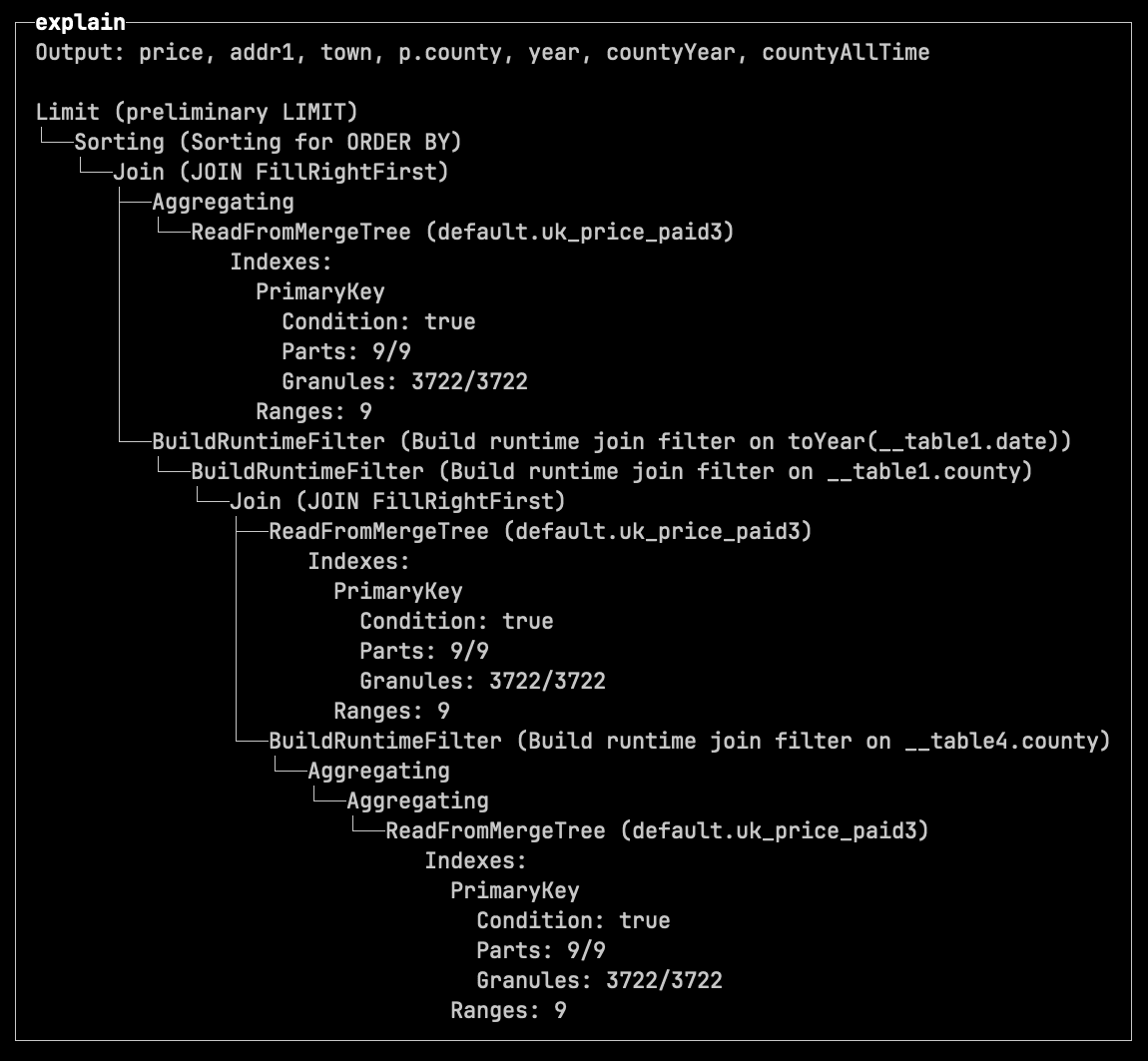
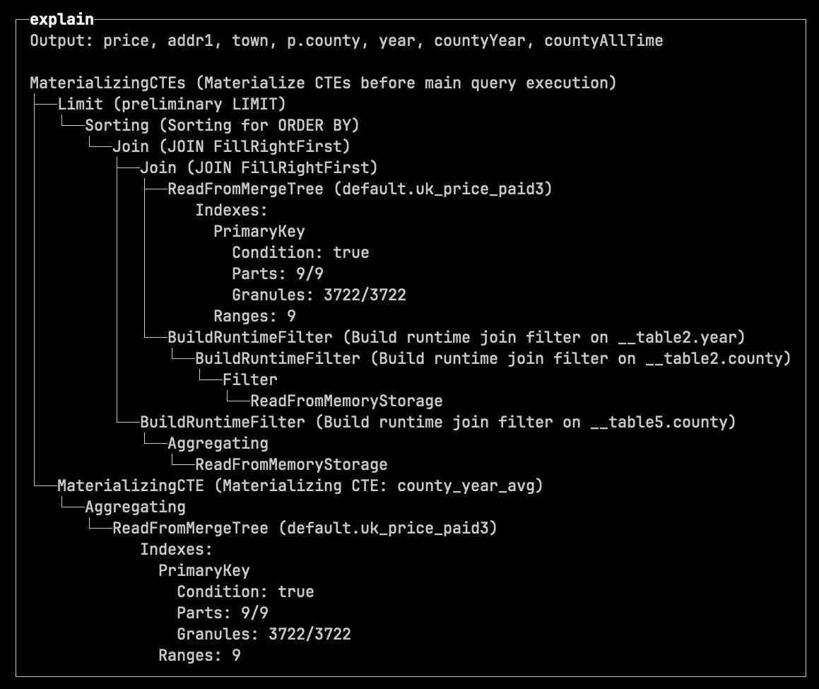
The 26.3 release also introduces new settings when using the EXPLAIN clause:
pretty=1 - tree-style indented output.compact=1 - collapses Expression steps.
If we prefix the query from the previous section with:
EXPLAIN indexes=1, pretty=1, compact=1
We see the following output for the not materialized CTE:
And the following output for the materialized one:
The naturalSortKey function enables human-friendly sorting.
For example, if we wanted to work out when Geospatial functions were added to ClickHouse, we could write the following query:
SELECT introduced_in, count()
FROM system.functions
WHERE categories LIKE '%Geo%'
GROUP BY ALL
ORDER BY introduced_in;
┌─introduced_in─┬─count()─┐
│ 1.1.0         │       5 │
│ 20.1.0        │      10 │
│ 20.3.0        │       6 │
│ 20.4.0        │       1 │
│ 21.11.0       │       4 │
│ 21.4.0        │      24 │
│ 21.9.0        │      11 │
│ 22.1.0        │       3 │
│ 22.2.0        │       5 │
│ 22.6.0        │      15 │
│ 25.10.0       │       4 │
│ 25.11.0       │       6 │
│ 25.12.0       │       1 │
│ 25.6.0        │       2 │
│ 25.7.0        │       2 │
└───────────────┴─────────┘
In the normal sort order, 21.11.0 comes before 21.4.0 and 21.9.0, which isn’t what we’d expect. We can use the new function to sort this data in the expected order:
SELECT introduced_in, count()
FROM system.functions
WHERE categories LIKE '%Geo%'
GROUP BY ALL
ORDER BY naturalSortKey(introduced_in);
┌─introduced_in─┬─count()─┐
│ 1.1.0         │       5 │
│ 20.1.0        │      10 │
│ 20.3.0        │       6 │
│ 20.4.0        │       1 │
│ 21.4.0        │      24 │
│ 21.9.0        │      11 │
│ 21.11.0       │       4 │
│ 22.1.0        │       3 │
│ 22.2.0        │       5 │
│ 22.6.0        │      15 │
│ 25.6.0        │       2 │
│ 25.7.0        │       2 │
│ 25.10.0       │       4 │
│ 25.11.0       │       6 │
│ 25.12.0       │       1 │
└───────────────┴─────────┘
Before ClickHouse 26.3, the JSONExtract function could only be used to extract fields from JSON strings, as shown in the example below:
WITH '{"ClickHouse":{"version":"26.3"}}' AS s
SELECT s, toTypeName(s), JSONExtractString(s, 'ClickHouse', 'version');
┌─s─────────────────────────────────┬─toTypeName(s)─┬─JSONExtractS⋯ 'version')─┐
│ {"ClickHouse":{"version":"26.3"}} │ String        │ 26.3                     │
└───────────────────────────────────┴───────────────┴──────────────────────────┘
If you tried to use this function to extract fields from a JSON type, you’d get the following exception:
WITH '{"ClickHouse":{"version":"26.3"}}'::JSON AS s
SELECT s, toTypeName(s), JSONExtractString(s, 'ClickHouse', 'version');
Received exception:
Code: 43. DB::Exception: The first argument of function JSONExtractString should be a string containing JSON, illegal type: JSON: In scope WITH CAST('{"ClickHouse":{"version":"26.3"}}', 'JSON') AS s SELECT JSONExtractString(s, 'ClickHouse', 'version'). (ILLEGAL_TYPE_OF_ARGUMENT)
If you run the same query in 26.3, it will return the following output:
┌─s─────────────────────────────────┬─toTypeName(s)─┬─JSONExtractS⋯ 'version')─┐
│ {"ClickHouse":{"version":"26.3"}} │ JSON          │ 26.3                     │
└───────────────────────────────────┴───────────────┴──────────────────────────┘
As of 26.3, you can now create user-defined functions (UDFs) in WebAssembly. You can write a UDF in any language that compiles to WASM. The execution of those functions is sandboxed with Wasmtime.
This is an experimental feature at the moment, so you’ll need to enable it at the server level:
config.d/webassembly.xml
<clickhouse>
   <allow_experimental_webassembly_udf>true</allow_experimental_webassembly_udf>
   <webassembly_udf_engine>wasmtime</webassembly_udf_engine>
</clickhouse>
Once you’ve done that, you’ll be able to see the registered WebAssembly UDFS by running the following query:
SELECT *
FROM system.webassembly_modules;
┌─name────┬─code─┬──────────────────────────────────────────────────────────────────────────hash─┐
│ collatz │      │ 72604391076586157580802760480449151909954051103190340835087306247242304166984 │
└─────────┴──────┴───────────────────────────────────────────────────────────────────────────────┘
You can follow the WebAssembly User-Defined Functions guide for a step-by-step example of this functionality.
In ClickHouse, every INSERT creates a new data part sorted by the table’s sorting key. To keep inserts fast, additional data processing is deferred to background part merges.
These merges run continuously, combining smaller parts into larger ones. In the process, ClickHouse not only improves data layout for data skipping, but also performs maintenance work such as replacing rows, deleting rows, updating rows, or pre-aggregating data.
To perform merges efficiently, ClickHouse automatically selects one of two merge algorithms based on factors such as table width, number of rows, and data size:
-
Reads and merges only the sorting key columns first
-
Temporarily records the final row order for the remaining columns
-
Then processes and writes remaining columns one by one
To see the difference more clearly, let’s look at how each merge strategy works in practice.
Horizontal merge: simple and CPU efficient
Horizontal merging is straightforward. Since all parts are already sorted by the same key, ClickHouse performs a single linear merge pass, similar to merge sort:
-
Parts are read sequentially
-
Rows are compared on the fly
-
A new merged part is written
The animation below illustrates this using example data parts from a table with a sorting key (town, street):
The animation shows the horizontal merge process in three steps:
① Merge blocks
Data from multiple parts is read in blocks and merged in memory based on the sorting key in a single linear merge pass. For simplicity, the animation shows full parts instead of block-by-block processing.
② Write blocks into a new part
The merged data is written into a new data part. Again, the animation shows this as a single step for simplicity.
③ Deactivate old parts
Once the merge is complete, the original parts are marked as inactive and eventually removed.
For wide tables (e.g. 100+ columns), this approach can be memory-intensive.
Because merges operate on row blocks, ClickHouse must load entire blocks of wide rows into memory. The wider the table, the more expensive this becomes.
To address this, ClickHouse uses an alternative merge strategy.
Vertical merging reduces memory usage by processing columns separately.
The animation below shows this for a table with a sorting key (town, street). For simplicity, only one additional column price is shown; other columns are processed the same way.
The animation shows the vertical merge process in five steps:
① Merge sorting key columns first
Data from multiple parts is read block by block and merged in memory using the sorting key in a single linear pass. For simplicity, the animation shows full columns instead of several column-blocks.
② Record row order and write key columns
The resulting final row order is temporarily stored, and the merged sorting key columns are written to the new data part.
③ Merge next column by recorded row order
The remaining columns are processed one by one. For each column, data is read block by block from all parts and merged according to the previously recorded final row order. The animation illustrates this as a single step and for one column only.
This combination of column-by-column and block-by-block processing is what makes vertical merges memory efficient.
④ Add column data to the new part
The merged column data is appended to the new data part after each column is processed.
⑤ Deactivate old parts
Once all columns are processed, the original parts are marked as inactive and eventually removed.
This merge strategy is more efficient for wide tables, where loading all columns at once would be memory-expensive.
In practice, ClickHouse uses vertical merges only when it is expected to be beneficial.
With default settings, vertical merge becomes eligible when the to be merged parts contain at least 131,072 rows in total or at least 11 non-primary-key columns.
In other words, for merges where the memory savings are expected to outweigh the extra bookkeeping, ClickHouse automatically switches to the more memory-efficient vertical merge algorithm.
This is often the case in TTL-driven workloads, where large volumes of data accumulate over time and are often stored in wide tables.
In ClickHouse, you can define TTL rules to automatically delete table data after a certain period.
This is particularly useful for data that naturally ages out, such as logs, events, telemetry streams, or rolling analytics datasets.
These workloads typically accumulate large volumes of data over time, and in modern observability use cases, that data is often stored as wide events, with each row containing a large number of attributes.
As a result, TTL-based deletions frequently operate on large, wide tables, where merge operations become memory-intensive.
As mentioned earlier, TTL DELETE is executed during background merges, even though it doesn’t combine parts, instead reading individual parts, filtering them by TTL rules, and rewriting them.
Starting with version 26.3, TTL DELETE operations can use vertical merges, reducing memory usage during these operations.
This behavior is controlled by the new vertical_merge_optimize_ttl_delete MergeTree setting (enabled by default).
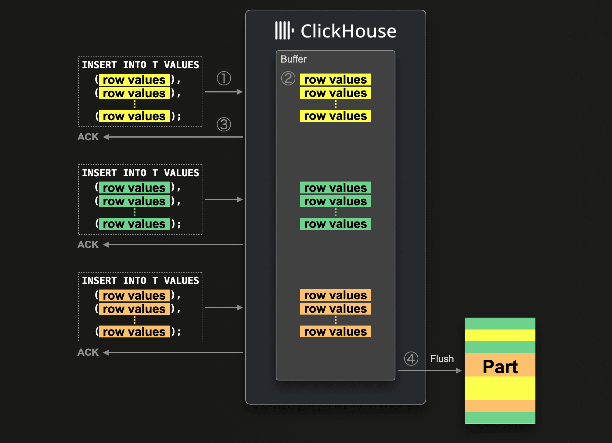
As described in the “Vertical merge for TTL DELETE” section above, ClickHouse achieves high insert throughput by writing independent data parts and merging them later in the background.
Creating and merging many small parts in a short time window is resource-intensive, so inserts should be batched for optimal performance.
Either client-side, or you can use asynchronous inserts in ClickHouse.
Asynchronous inserts shift data batching from the client side to the server side: data from insert queries is inserted into a buffer first and then written to storage during the next buffer flush, triggered by a timeout, accumulated data size, or number of inserts.
Since we originally blogged about asynchronous inserts, we refined and optimized them further.
For example, since 24.2, asynchronous inserts use an adaptive algorithm to automatically adjust the buffer flush timeout based on the frequency of inserts.
In version 26.1, we introduced a consistent deduplication mechanism for asynchronous inserts with materialized views.
And now, starting with 26.3 LTS, asynchronous inserts are enabled by default.
ClickHouse automatically batches small inserts, reducing the number of parts created by frequent writes, without requiring configuration changes for most users.
"When will you stop optimizing join performance?" We will never stop!
It’s not just asynchronous inserts that have come a long way. JOIN reordering has also seen significant improvements in recent months (and slightly related, just last month we improved the performance of RIGHT OUTER and FULL OUTER JOINs).
As a quick reminder, when multiple tables are joined, the join order does not affect correctness, but it can dramatically affect performance. Because different join orders can produce vastly different amounts of intermediate data. Since ClickHouse’s default hash-based join algorithms build in-memory structures from one side of each join, choosing a join order that keeps build inputs small is critical for fast and efficient execution.
JOIN reordering in ClickHouse has evolved significantly over recent releases:
-
Local automatic join reordering for two joined tables was introduced first, enabling the optimizer to move the smaller of both tables to the right (build) side and therefore reducing the effort needed to build the hash table. (24.12)
-
This was followed by global automatic join reordering, allowing efficient optimization of complex join graphs across dozens of tables and across the most common join types (inner, outer, cross, semi, anti). (25.09)
This resulted in significant improvements, for example, a 1,450× speedup and 25× reduction in memory usage on one TPC-H example query.
-
To further improve decision-making, ClickHouse introduced automatic column statistics, enabling better cost estimation for join ordering. (25.10)
-
Finally, a more powerful join reordering algorithm (DPsize) was added for INNER JOINs, exploring a larger space of join orders and often producing more efficient execution plans. (25.12)
ClickHouse can now reorder all major join types, including ANTI, SEMI, and FULL joins.
Previously limited to INNER and LEFT/RIGHT joins, the optimizer now automatically selects the most efficient build side across all major join types, producing better plans and reducing memory usage.
This relies on statistics being enabled for tables.
This release not only introduces “Vertical merges for TTL DELETE”, an optimization particularly useful for observability workloads, but also improves the internal storage of the ClickHouse Map data type, speeding up access patterns common in those workloads.
Observability data, such as OpenTelemetry (OTEL) events, often includes a large number of tags. These tags are simple key–value pairs that provide additional context for each recorded event.
Since tags are inherently flat, they don’t benefit from a datatype like JSON supporting deeply nested structures.
Instead, the Map data type, a collection of key–value pairs, maps naturally to the tags structure.
Internally, Map is Array(Tuple(Key, Value)) in ClickHouse. The diagram below shows how two rows inserted into a table with a tags column of type Map are stored on disk.
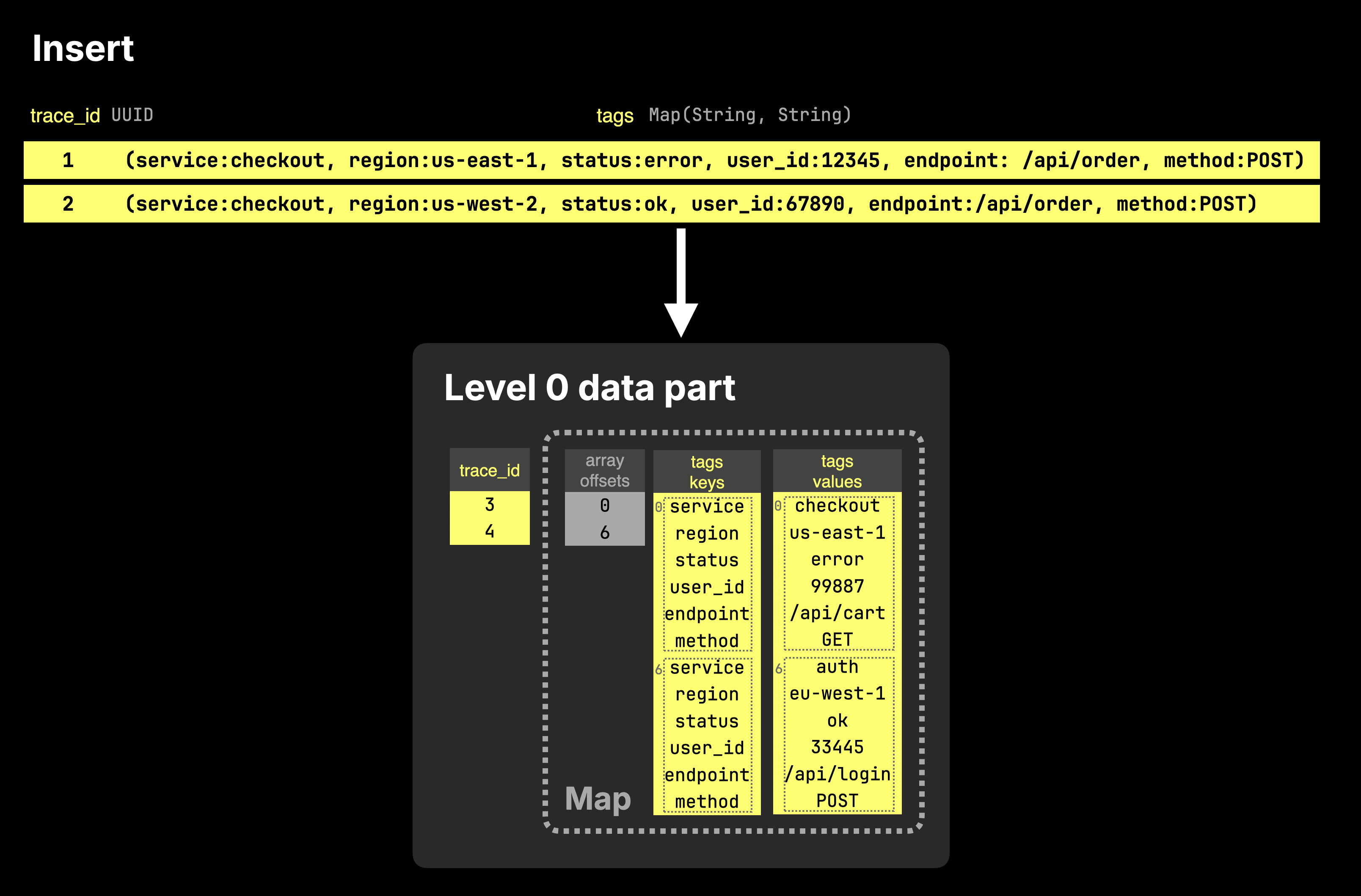
As the diagram shows, a Map column is stored on disk as two separate arrays: one containing all keys and one containing the corresponding values. These arrays are paired with an offsets file, which maps entries back to the table rows they belong to.
In practice, queries usually access only a small subset of keys within a map. Because keys and values are stored as plain arrays without indexing, every lookup requires scanning the arrays, leading to unnecessary data reads.
To address this, the new storage format splits map data into multiple sub-arrays by grouping keys into hash-based buckets. As a result, accessing a single key, such as tags['status'], requires reading only the corresponding bucket instead of the entire column.
This significantly reduces the amount of data processed for common lookup patterns.
Importantly, this optimization does not impact insert performance. New data is written using the existing format, and the bucketed layout is applied later during background merges.
The next diagram sketches this for two inserts into a table with a tags column of type Map.
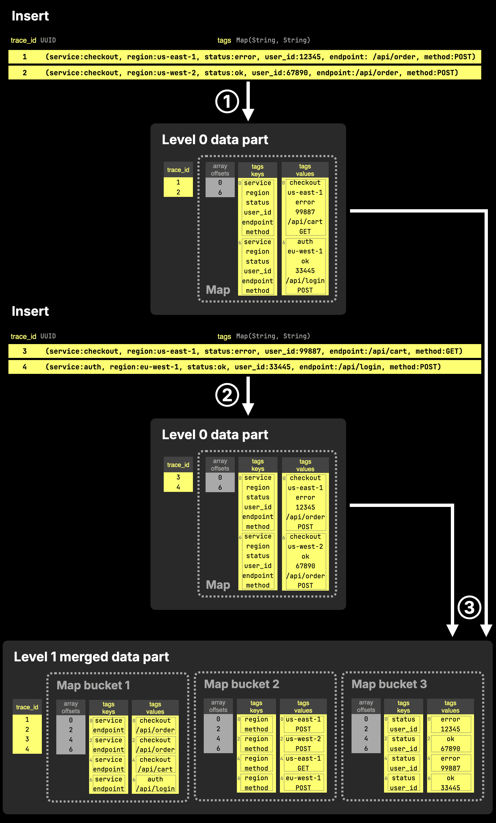
The diagram shows three steps:
① Insert → Level 0 parts (default format)
Each insert creates a new data part using the standard Map layout: keys and values are stored as two flat arrays, without any bucketing.
② Another insert → another Level 0 part
A second insert produces another part in the same format. At this stage, all map data is still stored as full key and value arrays.
Accessing a single key would require scanning the entire arrays, but this is typically not an issue since Level 0 parts are small.
③ Background merge → bucketed Map storage
During the next background merge, ClickHouse reorganizes the Map data by splitting keys into hash-based buckets. Each bucket stores a subset of keys and their corresponding values in smaller arrays.
When accessing a key such as tags['status'], ClickHouse uses the hash of the key to locate the corresponding bucket (e.g., bucket 3) and reads only those arrays, significantly reducing the amount of data that needs to be scanned.
In practice, this results in 2–49x faster single-key lookups depending on map size.
This behavior is controlled by the new map_serialization_version MergeTree setting set to with_buckets, and max_buckets_in_map specifies into how many buckets the data is split at a maximim (32 by default).
Additional settings further control the exact layout. In the example shown in the diagram above, the bucketed structure results from the following configuration:
- map_serialization_version_for_zero_level_parts = 'basic'
- map_serialization_version = 'with_buckets'
- max_buckets_in_map = 3
- map_buckets_strategy = 'const'
- map_buckets_min_avg_size = 0.


