TL;DR
We redesigned the ClickHouse full-text index to work efficiently on object storage.
The new layout favors sequential access and can answer many queries directly from the index without reading the indexed text column at all.
This post is a deep dive into the new design, written by the engineers who built it.
Full-text search in ClickHouse has gone through several iterations as we worked to bring fast, native text indexing to a columnar analytical database. Each iteration improved performance, usability, and integration with the query engine.
With ClickHouse Cloud, a new constraint appeared.
The text index must deliver the same high performance even when data is stored on object storage rather than on local disks.
Data reads and writes on remote object storage have fundamentally different performance characteristics. Designs that require random reads or frequent lookups of a few bytes become a bottleneck at scale.
We redesigned the new text index with these constraints in mind.
In this post, we first walk through the internal design of the new text index and how it is used by the query engine during full-text searches. In the second half, we move from implementation details to configuration and usage.
For a high-level overview of full-text search in ClickHouse and when to use it, see our GA announcement.
As discussed in our earlier work on caching in ClickHouse Cloud, latency (not bandwidth) is in practice the real bottleneck when data lives on remote object storage.
Object storage provides high throughput but significantly higher access latency than local disks.
The previous text index relied on scattered lookup patterns that were efficient on local disks but became slow on object storage, as many small, disjoint lookups amplify latency.
To maintain high performance on object storage, we redesigned the text index to favor sequential access patterns, allowing efficient use of object storage without regressing the performance of full-text search on local disks.
To see how this is implemented, we will now walk through all relevant index data structures, starting with how the index is stored on disk.
As a reminder, ClickHouse stores table data on disk as a collection of data parts.
Each data part contains a sparse primary index used for range pruning, and may also contain additional secondary data skipping indexes such as minmax, set, or bloom filter indexes.
The text index belongs to this second category of indexes. Like other data skipping indexes, it is defined per column whose textual content should be indexed for fast full-text search, and it is stored inside each data part alongside the column files and the primary index, as illustrated in the diagram below.
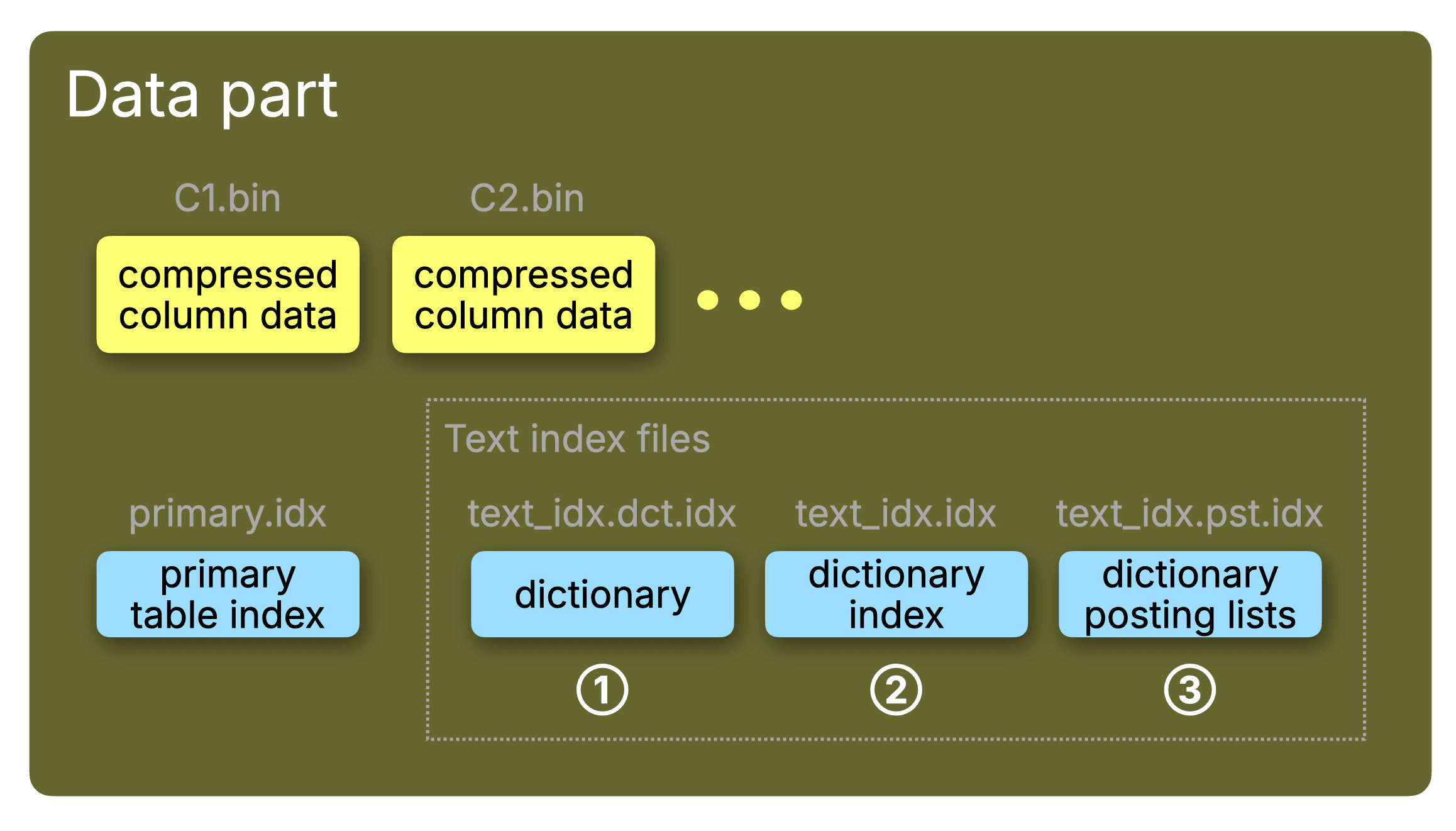
As shown in the diagram above, the text index internally consists of three main components, each of which is stored as a separate file per part:
① the dictionary file (text_idx.dct.idx)
② the sparse dictionary index file (text_idx.idx)
③ the posting list file (text_idx.pst.idx)
The filenames are used in the diagrams below for clarity.
We go through each of the index components one by one in the following sections.
The dictionary is the part of the text index that stores all indexed tokens, and for each token a reference to a corresponding posting list, representing all row positions that contain the token.
The dictionary in earlier text index versions was based on a data structure known as Finite State Transducer (FST) - essentially a trie with prefix and suffix compression. FSTs provides compact storage and fast lookups on local SSDs. However, FSTs also rely on many small random reads, which become incredibly inefficient when the index is stored on object storage.
This led us to redesign the dictionary layout with two goals: First, we wanted to favor sequential access patterns over random reads. Second, since random lookups cannot be entirely avoided in index lookups, we wanted to keep their number per query at least as small as possible. This keeps end-to-end query latencies small and predictable as the indexed datasets grow.
To achieve this, the new text index dictionary uses a block-based layout: tokens are sorted alphabetically and grouped into fixed-size blocks of dictionary_block_size entries (default 512).
This enables sequential reads, efficient compression, and fast access to posting lists, as described in the following sections.
The diagram below shows multiple dictionary blocks located at different offsets within the same dictionary file (text_idx.dct.idx).
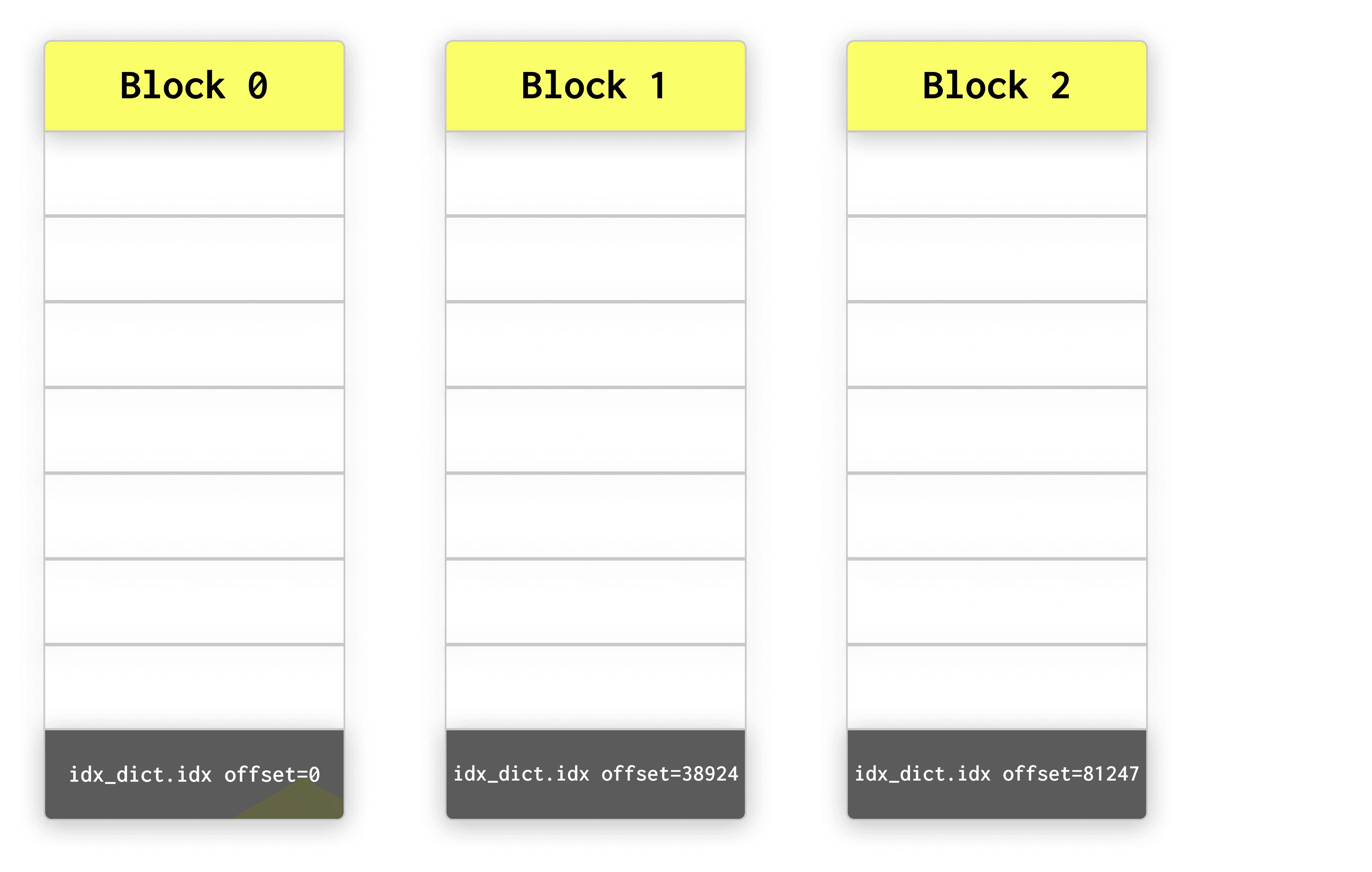
Each block is a self-contained chunk of sorted tokens that can be read sequentially.
Reading blocks sequentially avoids scattered random accesses and keeps lookups efficient even when the index files reside on object storage.
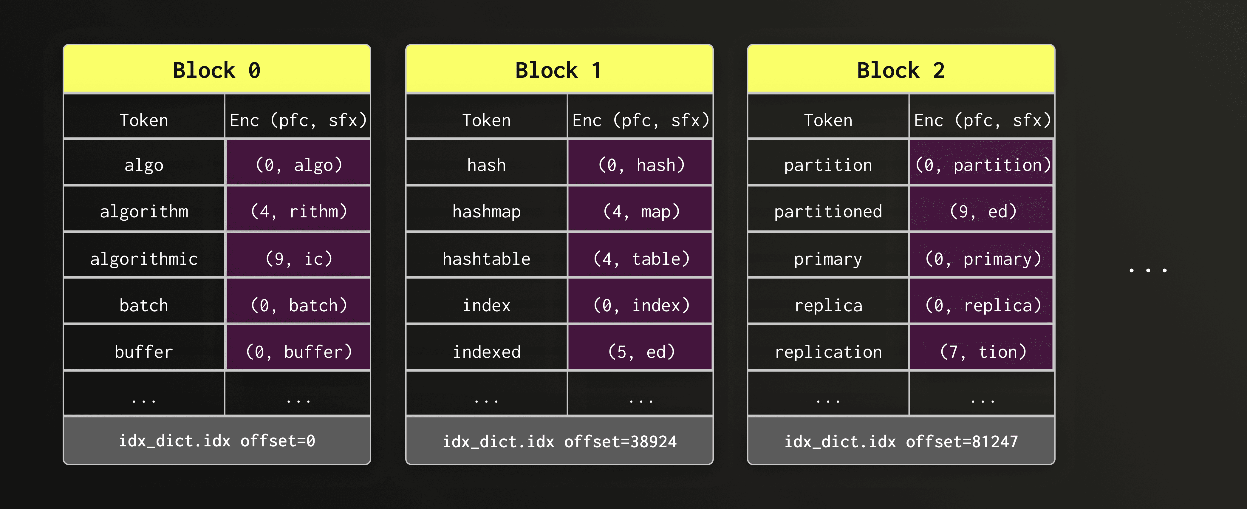
Looking at the blocks, we can immediately observe that consecutive tokens often share a common prefix — for example, "algo", "algorithm", and "algorithmic". Storing the full string for every token would be wasteful.
To keep dictionary blocks compact without forgoing the sequential layout, the new design compresses the tokens using front-coding. This compression method stores the first token of each block unchanged. All following tokens are each replaced by the length of the prefix they share with the previous token and their suffix.
Front-coding significantly reduces block size on disk.
In the diagram below, the token column is shown only for readability; on disk, only the encoded (prefix_length, suffix) values (highlighted in violet) are stored.
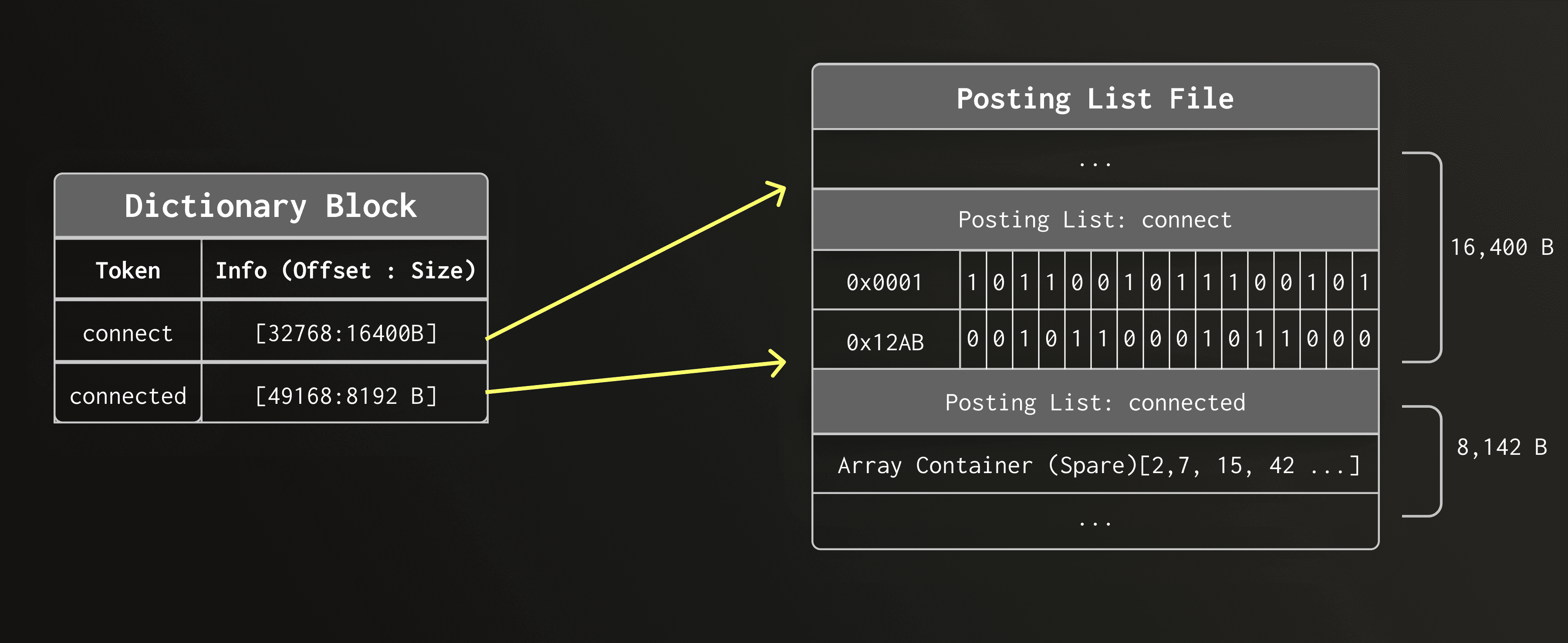
During text search, once a token is found in the dictionary, the engine must locate the rows where that token appears. These row positions of each token is stored in a posting list.
Each dictionary entry therefore stores a byte offset into the posting list file (text_idx.pst.idx), allowing ClickHouse to jump directly to the posting list of a token.
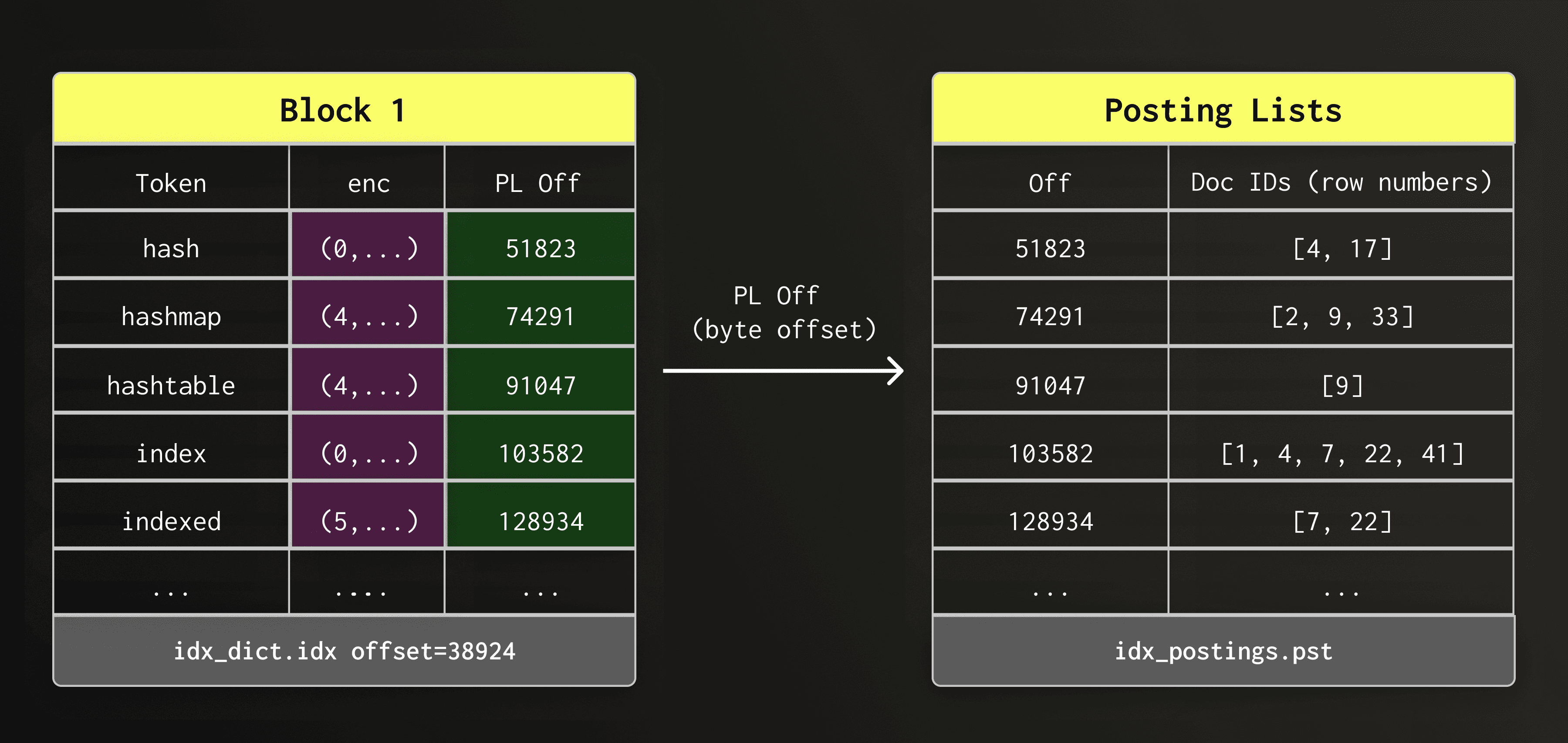
For simplicity, the diagram shows the data organization only conceptually; we implemented special cases for storing the actual posting lists which we describe in more detail later.
So far, we have looked at the dictionary layout, the first of the three main components that make up the new text index. Next, we look at the sparse index, which allows ClickHouse to find the correct dictionary block quickly without scanning the entire dictionary file.
With potentially millions of tokens spread across thousands of dictionary blocks, we need a fast way to find the right dictionary block that contains a given token.
Of course, we could load or scan all dictionary blocks (or do a binary search in them), but that would be unacceptably slow.
The sparse index solves this by recording the first token of each dictionary block together with the byte offset of this block within the dictionary file (text_idx.dct.idx).
The sparse index itself is stored in a separate file (text_idx.idx). Compared to the dictionary blocks and the posting lists, the sparse index is so small that it remains loaded in memory at all times.
The diagram below shows the sparse index file (text_idx.idx) pointing to dictionary blocks located at different offsets within the dictionary file.
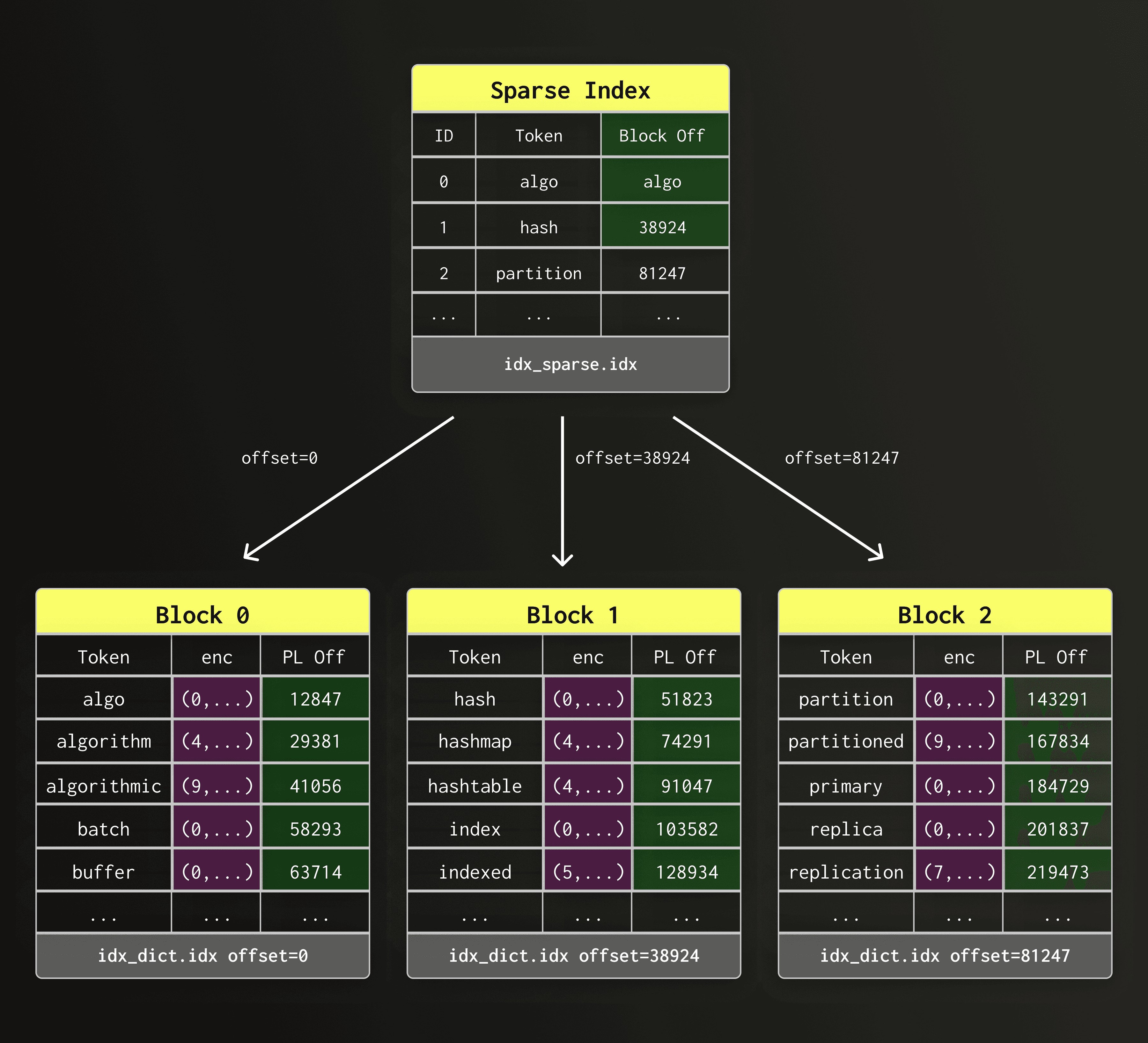
This design will look familiar to you if you know how ClickHouse's primary key index works — in fact, both indexes perform this kind of “sparse indexing”: they store for each block an entry point, allow to jump to the right neighborhood, and scan sequentially from there on. The difference is that, here, the blocks contain dictionary tokens instead of row values.
The sparse index and dictionary blocks minimize random I/O and allow lookups to proceed mostly sequentially, keeping dictionary access efficient on both local disks and object storage.
With the dictionary blocks and sparse index in place, the engine can locate a token efficiently.
The next step is to read the posting list, which stores the row positions on which a token appears.
In the previous section, we used a simplified layout to show how dictionary entries reference posting lists on disk.
In practice, posting lists can vary enormously in size. Some tokens appear only once or twice in the dataset, while others may appear in millions of rows.
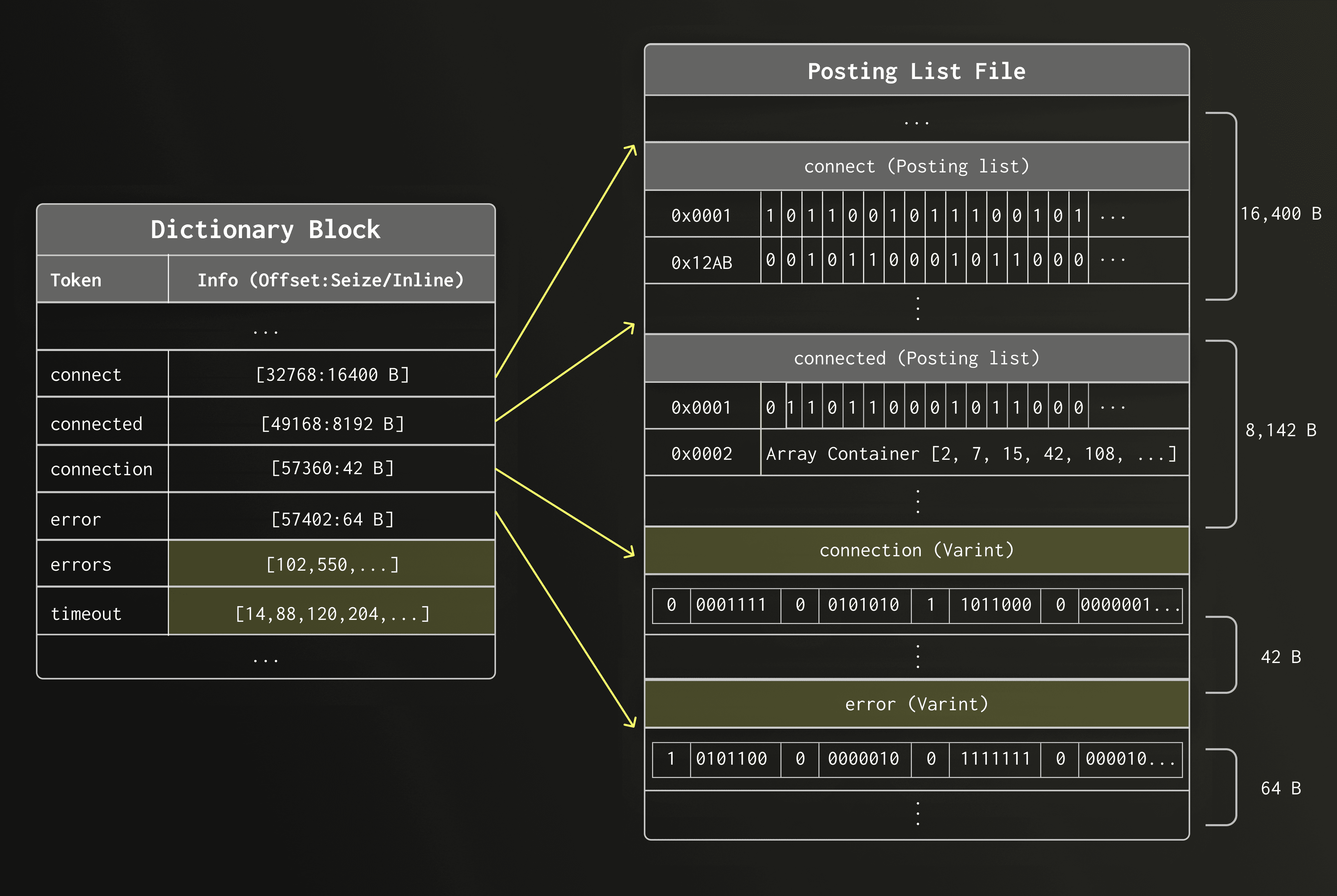
To represent posting lists of all sizes efficiently, the new text index in ClickHouse uses different posting list representations, depending on the posting list size:
- Roaring bitmap posting lists — used for posting lists with more than 12 row IDs
- VarInt-encoded posting lists — used for posting lists with 7 to 12 row IDs
- Embedded posting lists — used for posting lists with 6 or fewer row IDs
We describe each representation below.
A posting list with more than 12 contained rows is stored as a so-called Roaring Bitmap.
A Roaring Bitmap is a compressed bitmap that can hold a large set of 32-bit integers while still supporting fast intersections and unions. Both operations are important for SQL functions like hasAnyTokens() and hasAllTokens() that combine multiple posting lists.
Internal layout
Roaring Bitmaps split the 32-bit integer space into two halves. The upper half is based on the upper 16 bits of the row IDs, representing 65,536 different possible values.
The lower halves are stored in one of three different containers. Containers choose the most compact internal representation depending on the number of contained row IDs:
- Array container — used for sparse chunks
- Bitmap container — used for dense chunks
- Run-length container — used for chunks with many consecutive runs
This adaptive layout allows Roaring Bitmaps to compress posting lists with very different internal data distributions efficiently while still allowing for fast set operations.
Example
To see why this matters, consider the token connect in a large text dataset. Suppose connect appears in row IDs 65,536, 65,538, 65,539, 65,542, and tens of thousands more row IDs scattered across the table. Storing these numbers as a plain sorted array of 32-bit integers would cost 4 bytes per entry, that is ~200 KB just for storing 50,000 matching rows.
With Roaring Bitmaps, the upper 16 bits (0x0001) of each value identify the container — a bucket responsible for the row IDs in range 65,536–131,071. The lower 16 bits (0x0006) are the values stored inside that container. In this example, all four row IDs fall into the same container.
Each container independently chooses its internal layout based on the distribution of row IDs it contains:
On-disk layout
For large posting lists Roaring Bitmaps work extremely well: they provide good compression and enable efficient query operations such as intersecting multiple posting lists during search.
Internally, Roaring Bitmaps posting lists and are further divided into blocks (controlled by posting_list_block_size). Each block records the minimum and maximum row ID it contains. This metadata allows the query engine to skip decompressing blocks whose row ranges have already been ruled out by other predicates, reducing unnecessary work during search.
Limitations
However, Roaring bitmaps have a non-trivial minimum size due to their mandatory metadata. This overhead is negligible for large posting lists but it becomes wasteful for smaller posting lists. It is therefore important to introduce specialized representations for sparse tokens which are frequent in natural language and text datasets. ClickHouse’s inverted index uses two additional representations for such cases.
For small posting lists between 7 and 12 contained row IDs, the text index stores row IDs as a plain sequence of VarInt-compresed integers.
VarInt splits every byte into 7 bits of data “payload” bits and a continuation bit. As a result, values below 128 require only a single byte, values below 16,384 require two bytes, and so on.
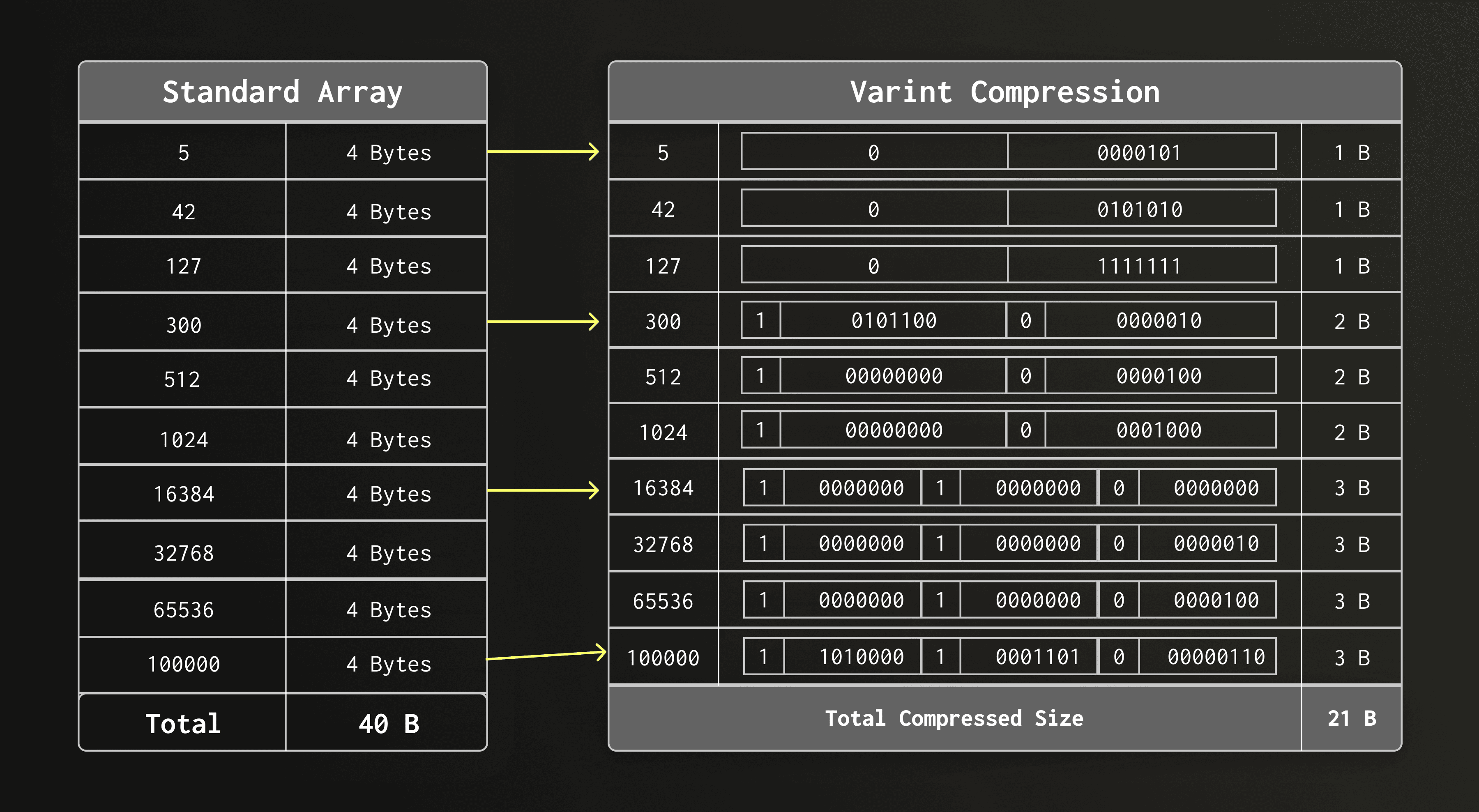
Because row IDs in small posting lists are often relatively small integers, this VarInt encoding compresses on average really well. For example, a posting list with 12 row IDs typically consumes only a few dozen bytes.
Why not use Roaring here
Using Roaring for such posting lists would be inefficient because the serialized structure has a minimum size of roughly 48 bytes caused by its header and container metadata. A simple list of VarInts is therefore the smaller and simpler alternative.
During development of the text index, we found that in real-world datasets, the vast majority of distinct tokens has very low cardinality. We looked at two large and very different datasets:
- 94.5%, respectively, 90.2% of all tokens appear in six or fewer rows.
- The median token cardinality is 2, respectively, 1.
- Only 3%, respectively, 6.1% of all tokens have a cardinality >12, i.e. the threshold below which Roaring Bitmaps have a static overhead.
- The threshold of six for embedded posting lists, chosen for memory layout reasons, turns out to capture 90% of tokens at P90 in both datasets (an accidental but near-perfect empirical fit).
Why storing small posting lists separately is wasteful
For most tokens, the full machinery of a Roaring Bitmap — with its container metadata and separate file entry — would constitute a significant overhead. For posting lists with six or less elements; the index could avoid writing into the posting list file entirely.
Embedded layout
Instead, if a token appears in six rows or fewer, the row IDs are embedded directly into the dictionary entry in place of the byte offset into the posting list file. As a result, the entire posting list can be read without an additional indirection and disk access.
Relation to small-object optimizations
This idea is inspired by the so-called small-object optimization (e.g. SSO, Short String Optimization) in systems programming, where very small values are stored inline rather than in a separate location. For rare tokens — which are extremely common in natural language datasets — this approach eliminates both the storage overhead and the extra I/O.
We have now covered the three main data structures of the new text index: dictionary blocks, the sparse index, and posting lists.
Before we look at how these pieces work together during query execution, we briefly detour into part merges, where the text index layout also plays an important role.
As mentioned earlier, the text index is stored inside each data part as three separate files: the dictionary, the sparse index, and the posting lists.
ClickHouse continuously merges smaller data parts into larger ones in the background, rewriting all files of the merged parts. When these files reside on object storage, merge performance depends heavily on the access pattern.
The new text index layout is designed to support efficient sequential access during merges. Because dictionary blocks are already stored in sorted order, the text index does not need to be rebuilt from scratch. Instead, ClickHouse can merge them using the same single merge pass that ClickHouse uses for table row data.
During the merge, the dictionaries of both parts are read sequentially and interleaved into a new sorted dictionary, avoiding random I/O and making index merges efficient even when index files reside on object storage.
The animation below shows a merge of two data parts. To keep the illustration focused, we only show the merge of the dictionary files, while the other files of the data part are merged in the same pass but not displayed.
Not shown in the animation above — posting lists in the posting list file (text_idx.pst.idx) are updated in the same pass by remapping row numbers using the row-id mapping produced during the main part merge, so the original text columns do not need to be read again.
As a result, merging text indexes is lightweight and scales with the size of the index itself, not with the size of the original text data.
Also not shown in the animation above — the sparse index file (text_idx.idx) is rebuilt for the merged part from the merged dictionary blocks.
With part merges covered, we now return to query execution and look at how the dictionary blocks, sparse index, and posting lists work together during search.
Consider the following table with a text index
CREATE TABLE docs
(
    `key` UInt64,
    `doc` String,
    INDEX idx(doc) TYPE text(tokenizer = splitByNonAlpha)
)
ENGINE = MergeTree()
ORDER BY key;
and the following query
SELECT count() FROM docs WHERE hasToken(doc, 'clickhouse');
Here, we are searching for a token clickhouse.
Let's walk through what happens internally when this query runs.
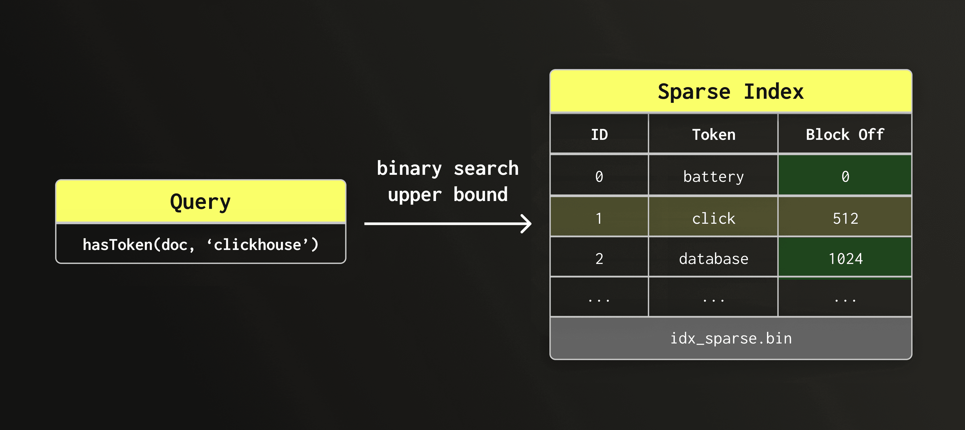
We first need to understand which dictionary block contains the token clickhouse.
Scanning all blocks sequentially would be too costly. Instead, we utilize the sparse index to find the right block.
Since the sparse index holds only the first token of each block, we run a binary search using the upper bound to locate the candidate block. The search token usually does not appear in the sparse index itself, but the upper bound tells us which block it would fall into if it was indexed.
Note that the sparse index is comparatively small and kept in main memory all the time. Therefore, the binary search itself takes only a few microseconds.
In the diagram below, the sparse index lookup returns the entry whose dictionary block may contain clickhouse. Its offset tells us which block to read from the dictionary file.
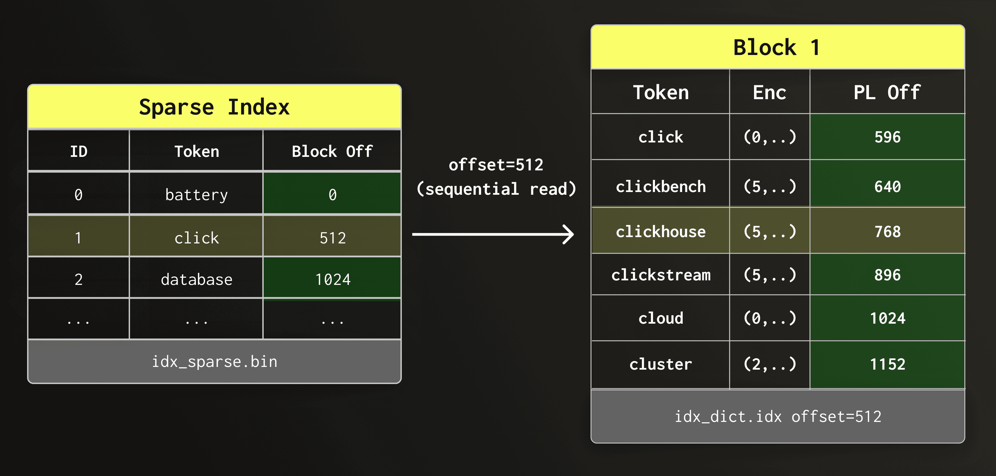
We next read the found dictionary block sequentially and scan its tokens.
Since the dictionary is stored on object storage, a block scan is about as fast as a point lookup in the block - the runtime is dominated by the latency to make a request and retrieve its result.
In the diagram below, the sparse index gives us the offset of the candidate dictionary block within the dictionary file. We read this block sequentially and scan it until clickhouse is found.
Once clickhouse is found in the dictionary block, we read the associated posting list from the posting list file.
In the diagram below, the candidate dictionary block gives us the offset of the posting list within the posting lists file. We then retrieve that posting list.
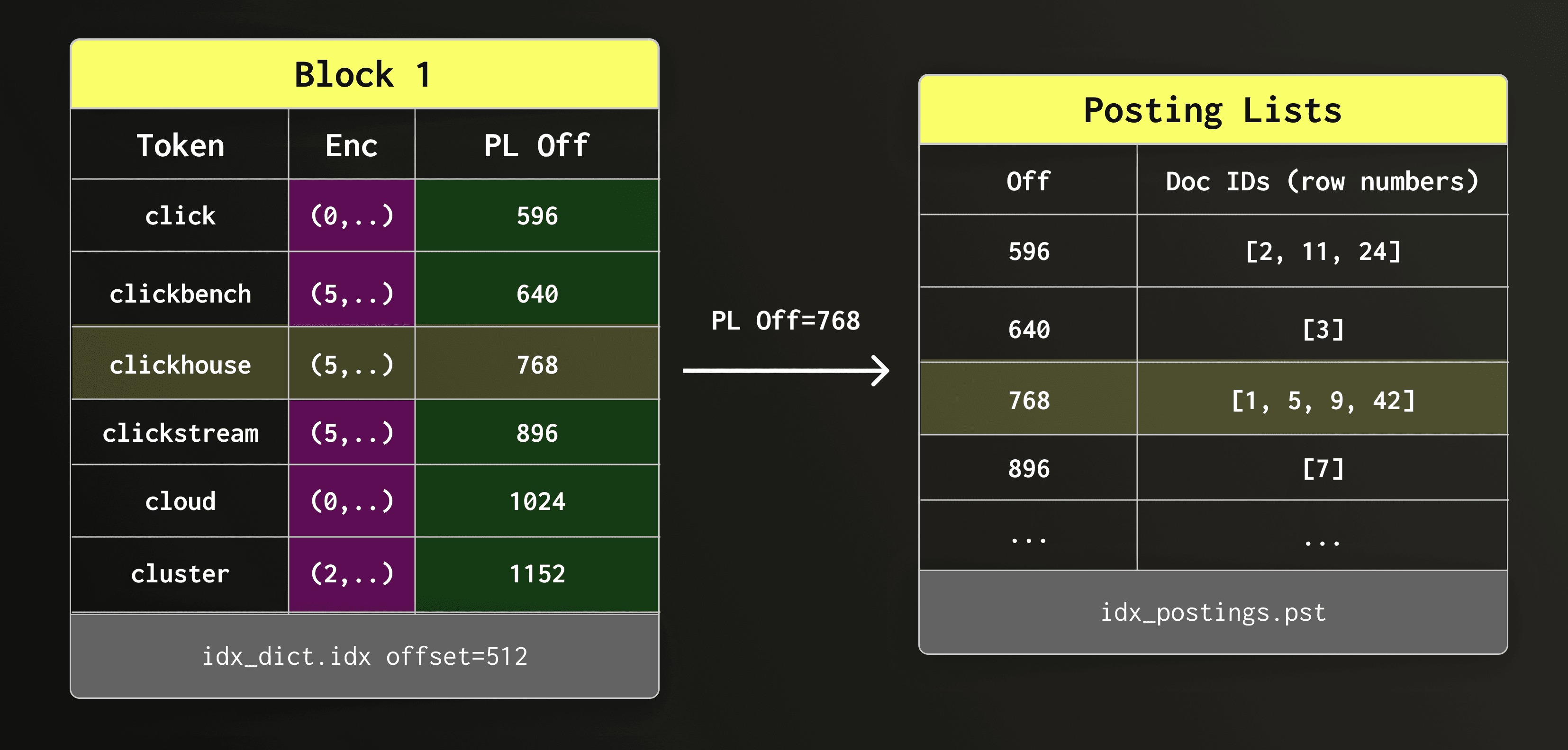
The retrieved posting list contains the matching row numbers.
The engine must now decide how to apply them during execution.
The index lookup returns the row numbers of matching rows as offsets inside data part columns.
Depending on the query shape and the text search functions used, ClickHouse can apply these offsets in three different ways, from most efficient to least efficient.
-
The engine can build a virtual column from the offsets and either
- avoid reading the indexed text columns entirely, or
- use the virtual column to narrow the candidate set before checking the remaining rows.
-
For more complex search patterns, it falls back to classical skip index evaluation, where the index is only used to skip granules that cannot contain matches.
In the following three sections, we describe these three approaches.
The text index is special among ClickHouse's skip indexes: its posting list contains the exact row numbers that match the query — no false positives, no further filtering needed.
Since we already know the exact rows, we can skip the usual filtering step and go straight to row-level masking.
Row-level masking with a virtual column
We use the row IDs in the posting list to construct an virtual boolean column (an internal column that only exists for the duration of the query) and set all matching rows to 1 and all other rows to 0.
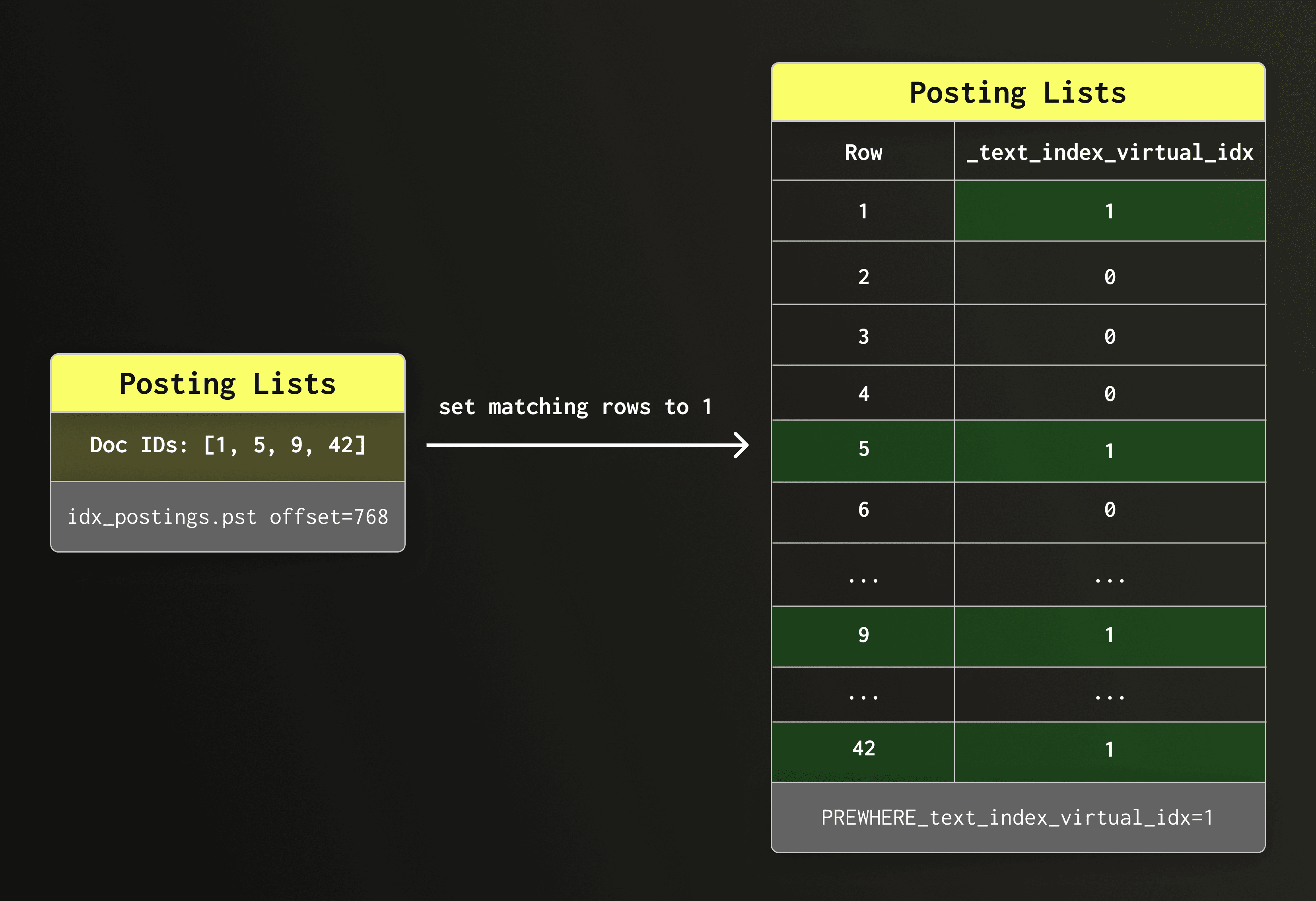
PREWHERE Query rewrite
ClickHouse then rewrites the query automatically to filter the virtual column. For example, query
SELECT count() FROM docs WHERE hasToken(doc, 'clickhouse');
is rewritten to
SELECT count() FROM docs PREWHERE _text_index_virtual_idx = 1;
PREWHERE evaluation
The PREWHERE clause evaluates its condition before other WHERE conditions are evaluated, meaning that only matching rows are passed to the next processing step (WHERE). Unmatched rows are eliminated as early as possible, reducing both I/O and the number of rows processed by subsequent operators.
Multiple tokens
When a query involves multiple tokens — for example, multiple hasToken conditions or a multi-token hasAnyTokens/hasAllTokens call — each token goes through the same lookup process independently, producing its own posting list. The virtual column is then filled using bitwise operations across these posting lists: AND for conjunctive conditions (all tokens must match), OR for disjunctive conditions (any token must match). This keeps the row filtering fast and avoids per-row string evaluation.
Why this is called direct read mode
What we just described is called “direct read” mode internally within ClickHouse. It is the most natural and most efficient way to utilize the text index.
The indexed text column is not read at all because the query is answered solely using the row-level information stored in the text index.
Limitations and supported functions
Direct read is only safe when the index tokens correspond exactly to the searched values and no false positives are possible.This is the case for SQL functions hasToken, hasAnyTokens, and hasAllTokens.
For certain predicates, normal direct read is not possible. For example, consider the query
SELECT col1, col2 FROM table WHERE col3 LIKE '%clickhouse performance%'
Using the index as a hint
To use the text index here, ClickHouse tokenizes the search pattern and looks up the tokens clickhouse and performance in the index. But a row containing both tokens is not guaranteed to match the full pattern. The words might appear far apart (clickhouse has great performance) or in a different order (the performance of clickhouse). In other words, relying just on the index alone can produce false positives. We can however use the index as a “hint” to rule out rows that don’t contain both tokens clickhouse and performance.
If most rows in a part do not contain both tokens, the index can eliminate the majority of candidates before the expensive LIKE evaluation runs on the column.
Direct read with hint mode
We call this “direct read with hint” mode - the virtual column narrows the candidate set, afterwards the original LIKE predicate is evaluated on the surviving rows.
Cost of reading posting lists
One challenge that comes with this trick is that reading posting lists is not free; it requires seeks and decompression. For example, if the token “clickhouse” appears in 80% of rows, the index would eliminate only relatively few rows, while still paying the I/O cost for all the rows. In that case it is better to avoid the index read entirely and evaluate the LIKE predicate directly on the column.
Selectivity-based decision
To make this decision, ClickHouse estimates the cardinality of the matching set using the per-token cardinalities already available from the dictionary, without reading any posting list payloads. If the estimate falls at or below text_index_hint_max_selectivity × N (default: 20% of total rows in the part), the hint is accepted: posting lists are read, the virtual column is filled, and non-matching rows are filtered before the LIKE check runs. Else, if the estimate exceeds the threshold, the hint is discarded: the virtual column is set to all-ones, no index I/O happens, and the original predicate carries the full filtering load.
Observability
The two outcomes are exposed as profile events — TextIndexUseHint and TextIndexDiscardHint — which can be observed in query logs to understand whether the index is contributing to a given query.
Supported functions
Supported SQL functions: like, startsWith, endsWith, mapContainsKeyLike/ValueLike
When a predicate cannot take any advantage of the direct read optimization or hint mode, the optimizer assigns it to execute in fallback read mode using ClickHouse’s skipping index infrastructure, and the predicate is evaluated normally against the column.
This technique is utilized for more complex patterns like: match, multiSearchAll, multiSearchAny.
Consider for example this query:
SELECT col1, col2 FROM table WHERE match(col3, 'connect.*timeout')
A regex predicate like this cannot be decomposed into a reliable set of tokens — the pattern expresses a sequence and proximity constraint that the index has no way to verify. The optimizer evaluates it in classical read mode:
The text index is used at a granule level by checking whether each granule contains tokens that could plausibly satisfy the pattern, and skipping those that cannot.
Why this is slower than direct read
For every granule that passes this coarse filter, the engine must decompress col3 in full and scan it row by row to evaluate the regex on the actual string data. Text columns are typically wide and expensive to decompress, and a pattern matching a common word can leave most granules as candidates. The index reduces I/O at the granule boundary, but the dominant cost (decompressing and scanning the column) remains.
This is precisely the gap that direct read closes for the predicates that support it: instead of decompressing the column to confirm what the index already knows, the posting list result is used directly.
At this point we have covered the internal design of the text index and how queries execute against it.
In the next section, we move from implementation details to configuration and usage.
If you want a quick practical introduction before diving into the details below, the short video below walks through how to create and use a text index in ClickHouse.
Before looking at how to create a text index, let’s first see which column types can be indexed.
A text index can be defined on columns of type String and FixedString, as well as Array and Map columns containing strings.
Nullable and LowCardinality strings are also supported, and all the aforementioned data types can be mixed and matched, e.g. Array(Nullable(FixedString)).
Let's now see how to create a text index.
There are two ways to add an index to a table, during table creation as part of the CREATE TABLE query or by running ALTER QUERY on an existing table. The index parameters are the same for both methods. See the documentation for more details.
Syntax:
CREATE/ALTER TABLE
...
   INDEX text_idx(str) TYPE text(
                               -- Mandatory parameters:
                               tokenizer = splitByNonAlpha
                                           | splitByString[(S)]
                                           | ngrams[(N)]
                                           | sparseGrams[(min_length[, max_length[, min_cutoff_length]])]
                                           | array
                               -- Optional parameters:
                               [, preprocessor = expression(str)]
                               -- See documentation for optional advanced parameters
				    ...
                           )
...
For example:
CREATE TABLE my_table
(
   key UInt64,
   str String,
   INDEX text_idx(str) TYPE text(tokenizer = ‘splitByNonAlpha’,
preprocessor = lower(str))
)
ENGINE = MergeTree
ORDER BY key
This creates a text index that will first lowercase any strings inserted into the ‘str’ column and then split them on non-alphanumeric characters and store them in the search-optimized text index structure described above. E.g. ‘HeLlo my1!!!NAME&is,234234’ will be split into [‘hello’, ‘my1’, ‘name’, ‘is’, ‘234234’] and will allow fast searching for these tokens.
Before we do any searching, let’s first take a look at the index parameters, specifically the tokenizer and preprocessor.
Index parameters and tokenization
Tokenization and preprocessing are two critical aspects of the text index that set it apart from other indexes and enable easy, fast searching over noisy text data. Together, these two components allow powerful, automated data transformation on INSERT, and can facilitate intuitive search results such as searching for cafe and matching ‘cafe’, ‘café’, ‘Café’, ‘CAFÉ’, etc.!
Let’s look at them in more detail.
This the proprocessor is executed on the input column prior to tokenization. Unlike functions applied directly to the input column when creating the index (e.g. INDEX idx(lower(col))), ClickHouse automatically applies preprocessor expressions also to the input in specialized text search functions (when run on the same indexed column): hasToken, hasAllTokens, and hasAnyTokens. When combined with ClickHouse’s extensive list of string functions we get a powerful preprocessing pipeline that can lowercase text, remove accents, process HTML, apply UTF8 normalization, and more!
The syntax for the pre-processor is as follows:
preprocessor = expression(<column-name>)
Some notes:
expression() can be as simple or complex as desired, it can contain any number of nested functions (although keep in mind that they will be run on each inserted row).- The expression functions **must **be deterministic.
<column-name> must match the index definition, aka if your index was defined with INDEX <idx-name>(lower(col1)) then the preprocessor expression must also be called on lower(col1), this is enforced.
Scenario 1: Input data is human-generated text, containing mixed-case characters and punctuation. The index lowercases the text, allowing for case-insensitive matching during search.
preprocessor = lower(col)

Input:       'Hello World! My_Name IS John123'
Preprocessed: 'hello world! my_name is john123'
Scenario 2: Input data contains multi-line strings, but only the first string is relevant for search.
preprocessor = substringIndex(col, '\n', 1)

Input:       'Hello World\nSecond Line\nThird Line'
Preprocessed: 'Hello World'
Scenario 3: Input data consists of HTML strings, the preprocessor is used to first remove HTML elements (replacing them with whitespace), then the result is lowercased.
preprocessor = lower(extractTextFromHTML(col))

Input: '
Hello World

My Name IS Sarah456

'
Preprocessed: 'hello world my name is sarah456'
Scenario 4: Input data contains mixed-case, accented text (e.g. French, German, etc.). First case folding is applied to the text, then the resulting text is stripped of diacritics (accents).
preprocessor = removeDiacriticsUTF8(caseFoldUTF8(col))

Input:       'Héllo Wörld ÑOÑO Ångström'
Preprocessed: 'hello world nono angstrom'
With preprocessing in place, we now look at tokenization, which defines how the input text is split into tokens for indexing.
This is the final piece of the puzzle, the tokenizer specifies how the column rows should be split into tokens. This is a critical decision because it will affect which queries match the index and which don’t. For example, an index that splits the data by whitespace will not match parts of words (e.g. ‘caf’ will not match ‘cafe’) but an index using the ngram tokenizer with an ngram length of 3 will match ‘caf’ to ‘cafe’.
There are a few broad types of tokenizers:
The ‘splitByNonAlpha’ and ‘splitByString’ tokenizers, as their names suggest, split the input by non-alphanumeric characters or custom separators. This is useful for most natural language text such as product reviews, or for splitting domain-specific strings with consistent delimiters.
Examples:
-- splitByNonAlpha
‘hello my1!!!name&is,234234’ -> [‘hello’, ‘my1’, ‘name’, ‘is’, ‘234234’]

-- splitByString with default ' ' separator
'hello my name is John' -> ['hello', 'my', 'name', 'is', 'John']

-- splitByString with custom separators [', ', '; ', '\n']
'apples, oranges; bananas\npears' -> ['apples', 'oranges', 'bananas', 'pears']

-- splitting csv data (custom separator ',')
'hello,world,foo,bar' -> ['hello', 'world', 'foo', 'bar']
The ‘ngrams’ and ‘sparseGrams’ tokenizers split strings into constant-length and variable-length tokens, respectively. The ngram length for the ‘ngrams’ tokenizer can be specified using an optional integer parameter between 1 and 8, for example, tokenizer = ngrams(3). The default ngram size, if not specified explicitly, is 3. The sparseGrams function uses a special algorithm to output variable-length ngrams controlled by the min_ngram_length and max_ngram_length parameters, see the sparseGrams function documentation for more information.
Examples:
-- ngrams (default size 3)
'hello' -> ['hel', 'ell', 'llo']

-- ngrams (size 4)
'hello' -> ['hell', 'ello']

-- sparseGrams (default min_length=3, max_length=100)
'hello' -> ['hel', 'hell', 'hello', 'ell', 'ello', 'llo']
The array tokenizer performs no tokenization, i.e. every row value is treated as a token (see function array).
'hello my name is John' -> ['hello my name is John']
Coming soon, the unicodeWord tokenizer will split ASCII characters in a consistent, default manner, as well as splitting each non-ASCII Unicode character into its own token. This provides basic tokenization support for non-whitespace-delimited languages such as Chinese, Japanese, Korean, and others.
'Hello世界' -> ['Hello', '世', '界']
All available tokenizers are listed in system.tokenizers, however this also lists the now deprecated bloom filter indexes tokenbf_v1 and ngrambf_v1, which are no longer recommended due to being less versatile, less performant, and harder to use than the text index.
With the index in place, we can now look at how to use it in search queries.
The part you’ve all been waiting for! Now that we have an index set up on a column, let’s populate it with some data and try searching for some text!
While common string search functions such as =, IN, and LIKE (the full list is provided further down) will leverage the text index by default, we recommend using the new text search functions hasAnyTokens and hasAllTokens for best results.
Functions hasAnyTokens and hasAllTokens match against one or all of the given tokens, respectively. These functions are tailor-made to work with the text index, and since they have no legacy behavior that must be maintained they are able to use all new text index features, such as the preprocessor, by default.
These two functions accept the search tokens as either a string, which will be preprocessed and tokenized using the same preprocessor and tokenizer used for the index column, or as an array of already processed tokens to which no preprocessing/tokenization will be applied prior to searching.
Creating and populating the table and index.
CREATE TABLE articles
(
    key    UInt64,
    str    String,
    INDEX  text_idx(str) TYPE text(tokenizer = 'splitByNonAlpha', preprocessor = lower(str))
)
ENGINE = MergeTree
ORDER BY key;

INSERT INTO articles VALUES
    (1, 'ClickHouse is FAST'),
    (2, 'fast cars and SLOW trains'),
    (3, 'The Quick Brown Fox'),
    (4, 'CLICKHOUSE is Scalable');
Using hasAny/AllTokens with the input as a string, preprocessing and tokenization will be applied before searching.
SELECT key, str
FROM articles
WHERE hasAnyTokens(str, 'ClickHouse');

-- Result:
-- ┌─key─┬─str───────────────────┐
-- │   1 │ ClickHouse is FAST    │
-- │   4 │ CLICKHOUSE is Scalable│
-- └─────┴───────────────────────┘

SELECT key, str
FROM articles
WHERE hasAllTokens(str, 'clickhouse FaSt');

-- Result:
-- ┌─key─┬─str────────────────┐
-- │   1 │ ClickHouse is FAST │
-- └─────┴────────────────────┘
Using the array overload, the tokens are NOT preprocessed and NOT tokenized, search is performed using the array strings as-is.
-- Notice that while 'slow' matches (since 'SLOW' was stored as 'slow' in the index), 'FAST' in row 1 does not match, despite matching the un-pre-processed text in the column, since it was stored in the index as 'fast' and 'FAST' != 'fast'.
SELECT key, str
FROM articles
WHERE hasAnyTokens(str, ['FAST', 'slow']);

-- Result:
-- ┌─key─┬─str───────────────────────┐
-- │   2 │ fast cars and SLOW trains │
-- └─────┴───────────────────────────┘

-- The below example only matches because the format of the input tokens is the same as that of the preprocessed and tokenized index rows.
SELECT key, str
FROM articles
WHERE hasAllTokens(str, ['quick', 'fox']);

-- Result:
-- ┌─key─┬─str─────────────────┐
-- │   3 │ The Quick Brown Fox │
-- └─────┴─────────────────────┘
Here is a fiddle link with the above examples: https://fiddle.clickhouse.com/6bde1e09-4ef7-41f6-844f-7c2386a48399
Note that when provided as a string, the search tokens do not necessarily need to be in the same format as the text in the original column, this allows case- and accent-insensitive search, search over HTML without dealing with tags, and many other flexible ways of searching, all without modifying the original data, which will be returned in its original form!
The ngrams tokenizer breaks text into overlapping character sequences at index time, enabling partial-word and substring matching. This is particularly useful for searching over technical terms, product names, or identifiers where users may only know part of a word.
Creating and populating the table and index.
CREATE TABLE packages
(
    key    UInt64,
    str    String,
    INDEX  text_idx(str) TYPE text(tokenizer = 'ngrams', preprocessor = lower(str))
)
ENGINE = MergeTree
ORDER BY key;
INSERT INTO packages VALUES
    (1, 'ClickHouse - fast OLAP database'),
    (2, 'PostgreSQL - advanced relational database'),
    (3, 'Elasticsearch - distributed search engine'),
    (4, 'ClickHouse Cloud - serverless ClickHouse');
Search for rows containing a partial word — 'elastic' will match 'Elasticsearch', and 'house' will match both 'ClickHouse' rows.
SELECT key, str
FROM packages
WHERE hasAnyTokens(str, 'elastic house');
-- Result:
-- ┌─key─┬─str───────────────────────────────────────┐
-- │   1 │ ClickHouse - fast OLAP database           │
-- │   3 │ Elasticsearch - distributed search engine │
-- │   4 │ ClickHouse Cloud - serverless ClickHouse  │
-- └─────┴───────────────────────────────────────────┘
Require multiple partial tokens to all be present using hasAllTokens.
SELECT key, str
FROM packages
WHERE hasAllTokens(str, 'postgres sql');
-- Result:
-- ┌─key─┬─str─────────────────────────────────────────┐
-- │   2 │ PostgreSQL - advanced relational database   │
-- └─────┴─────────────────────────────────────────────┘
Note that ngrams indexes are larger than word-based indexes such as splitByNonAlpha, and may produce more false positives at the index scan stage (though query results are always exact). They are best used when partial-word matching is genuinely required rather than as a default choice.
The array tokenizer is a natural fit for columns already of type Array(String) — each array element becomes one token, with no preprocessor needed. This is the ideal choice for tag-style data that is stored as a proper array, and importantly, it preserves multi-word tags like 'machine learning' or 'distributed systems' as atomic tokens, which whitespace-based tokenizers like splitByNonAlpha would break apart.
Creating and populating the table and index.
CREATE TABLE job_listings
(
    key  UInt64,
    tags Array(String),
    INDEX text_idx(tags) TYPE text(tokenizer = 'array')
)
ENGINE = MergeTree
ORDER BY key;
INSERT INTO job_listings VALUES
    (1, ['rust', 'distributed systems', 'database']),
    (2, ['golang', 'machine learning', 'distributed systems']),
    (3, ['rust', 'machine learning', 'data engineering']),
    (4, ['python', 'data engineering', 'database']);
Find listings tagged with any of a set of tags using hasAnyTokens.
SELECT key, tags
FROM job_listings
WHERE hasAnyTokens(tags, ['rust', 'golang']);
-- Result:
-- ┌─key─┬─tags───────────────────────────────────────────────┐
-- │   1 │ ['rust','distributed systems','database']          │
-- │   2 │ ['golang','machine learning','distributed systems']│
-- │   3 │ ['rust','machine learning','data engineering'].    │
-- └─────┴────────────────────────────────────────────────────┘
Find listings that must have all of a set of tags using hasAllTokens.
SELECT key, tags
FROM job_listings
WHERE hasAllTokens(tags, ['machine learning', 'distributed systems']);
-- Result:
-- ┌─key─┬─tags───────────────────────────────────────────────┐
-- │   2 │ ['golang','machine learning','distributed systems']│
-- └─────┴────────────────────────────────────────────────────┘
Since the tags are already properly structured as an array, the array overload of hasAnyTokens and hasAllTokens is the natural choice here — the search tokens are passed as an array directly, with no preprocessing or tokenization applied, matching exactly against the indexed elements. However, note that here we need to be careful about the case of our search tokens. Since we did not preprocess the column data at all, only tokens that are the same case as the input will match. If we know our data is already lowercased, this is fine, but we must still be careful to then search for only lowercased tags.
One question that may arise after examining the above example, is if our data is already in an array and tokenized, why would we bother adding it to a text index? The answer, of course, is performance. Below is an example of the speedup gained from adding the text index to a relatively small table of 10 million rows.
-- Create table
CREATE TABLE job_listings
(
    `key` UInt64,
    `tags` Array(String)
)
ENGINE = MergeTree
ORDER BY key;
-- Insert 10 million rows of random arrays of 5 strings
INSERT INTO job_listings SELECT
    number,
    arrayMap(x -> (['rust', 'distributed systems', 'database', 'golang', 'machine learning', 'data engineering', 'python'][(rand((number * 7) + x) % 7) + 1]), range(5))
FROM numbers(10000000);

10000000 rows in set. Elapsed: 13.501 sec. Processed 10.00 million rows, 80.00 MB (740.71 thousand rows/s., 5.93 MB/s.)
Peak memory usage: 383.27 MiB.
-- Search without an index
SELECT count()
FROM job_listings
WHERE has(tags, 'machine learning');

   ┌─count()─┐
1. │ 5373152 │ -- 5.37 million
   └─────────┘

1 row in set. Elapsed: 0.198 sec. Processed 10.00 million rows, 1.02 GB (50.49 million rows/s., 5.13 GB/s.)
Peak memory usage: 50.27 MiB.
-- Add an index using ALTER TABLE
ALTER TABLE job_listings
    (ADD INDEX text_idx tags TYPE text(tokenizer = 'array') GRANULARITY 100000000);
-- Materialize the index on existing data, this takes a while but is a one-time op
ALTER TABLE job_listings
    (MATERIALIZE INDEX text_idx)
SETTINGS mutations_sync = 2;
-- Search with the index, achieving a speedup of more than 7x!
SELECT count()
FROM job_listings
WHERE hasAllTokens(tags, ['machine learning']);

   ┌─count()─┐
1. │ 5373152 │ -- 5.37 million
   └─────────┘

1 row in set. Elapsed: 0.027 sec. Processed 10.00 million rows, 10.00 MB (368.23 million rows/s., 368.23 MB/s.)
Peak memory usage: 5.42 MiB.
Beyond hasAnyTokens and hasAllTokens, the text index also accelerates a number of other functions, though these predate the index and don't support preprocessor expressions:
= — exact full-value matching; only useful with the array tokenizerIN — same as above but for multiple termsLIKE / match — pattern matching; only works with splitByNonAlpha, ngrams, or sparseGrams, and only when complete tokens can be extracted from the pattern (e.g. '% clickhouse %' not '%clickhouse%', a query with '%word1 word2 word3%' will use the index to search for 'word2' and then fall back to a brute force search on matching rows for the rest of the pattern.)startsWith / endsWith — similar token-extraction requirement as LIKE, will benefit from the index if the function can extract whole words, e.g. startsWith(col, word1, word2) will use the index to search for word1 and then will fall back to brute force search for the rest of the pattern. However, startsWith(col, word1 word2) (note the extra space!) will use the index for both words.hasToken / hasTokenOrNull — matches a single pre-tokenized token; does not tokenize the needle, and does not support preprocessorshas — matches a single token in an Array(String) columnmapContains / mapContainsKey — matches against map keys; requires an index on mapKeys(map)mapContainsValue — matches against map values; requires an index on mapValues(map)mapContainsKeyLike / mapContainsValueLike — pattern matching on map keys/valuesmap['key'] = value — index is used if defined on mapKeys or mapValues
For full details, see the documentation. For a graph of functions and which indexes they support, see this page. Note that negation functions (!=, NOT IN, NOT LIKE) are not supported for the text index, as it only keeps track of words/postings lists that do exist in the table.
With the current functionality covered, let’s take a look at what’s next for the text index.
We are not done yet. We are currently working on support for indexing JSON columns, faster evaluation of LIKE and regular expression patterns, improved text processing, and phrase search, where the index not only knows whether a token appears in a row, but also where it appears.
With that look at what’s coming next, let’s see what the new text index already delivers today, and what this means for ClickHouse Cloud users.
After multiple iterations and significant performance work, the text index in ClickHouse now delivers the same high-performance full-text search whether data is stored on local disks or on object storage.
The new index layout favors sequential access patterns and allows many predicates to be resolved directly from the index without reading the indexed text columns from disk.
In ClickHouse Cloud, the new index benefits from the same architecture that powers other large-scale workloads. Parallel replicas can fan out full-text queries across many nodes, the distributed cache keeps hot index data close to compute, and shared object storage allows all nodes to access the same index files without reshuffling data.
The result is that full-text search scales the same way as the rest of ClickHouse Cloud: add nodes, and queries get faster.
Stay tuned for the benchmarking post, where we compare the new text index with traditional text search engines and show why it replaces the older Bloom filter–based approach for text-heavy workloads.


