ClickHouse is an open-source columnar database management system designed for real-time analytical queries on massive datasets. It excels at aggregating billions of rows in milliseconds, making it a popular choice for analytics platforms, observability systems, real-time dashboards, and data warehouses. ClickHouse achieves this through its columnar storage format, aggressive compression, and vectorized query execution, but getting optimal performance requires understanding how to work with its architecture.
While ClickHouse is remarkably fast out of the box, poorly designed schemas, inefficient queries, or suboptimal configurations can leave significant performance on the table. A table that could return results in milliseconds might take seconds. Storage that could compress 50x might only achieve 10x. The difference often comes down to understanding how ClickHouse stores, compresses, and queries data and applying the right techniques to align your use case with its strengths.
Whether you're inserting billions of events per day, running complex analytical queries, or trying to reduce storage costs, the right optimizations can dramatically improve both performance and efficiency. Small changes to data types, table engines, or sorting keys can yield order-of-magnitude improvements.
In this post, I'll share 10 best practices that I've found make the biggest difference in my work as a Solutions Architect at ClickHouse, working hands-on with customers every day. These aren't theoretical recommendations, they're the patterns I find myself coming back to repeatedly across deployments of various shapes and sizes, covering topics from schema design and data modeling to query optimization and monitoring.
Using ClickHouse with AI agents?
If you're querying ClickHouse from an AI agent or LLM application, check out ClickHouse best practices for AI agents for guidance tailored to that use case.
1. Choose the Right Primary Key and Order By #
In ClickHouse, the ORDER BY clause in your table definition is one of the most important decisions you'll make. It determines how data is physically sorted in storage, which directly controls how efficiently queries can skip irrelevant data through primary index pruning. It also impacts compression efficiency since sorted data compresses far better as adjacent rows often share similar values.
When ClickHouse writes data, it sorts rows based on your ORDER BY columns and stores in memory the first values of each granule (by default 8,192 rows). At query time, filters on those columns allow ClickHouse to skip entire granules that can't contain matching data.
The key is aligning your ORDER BY with your most common query patterns. Put low-cardinality columns like tenant_id, region, or category first, followed by time-based columns. Avoid leading with high-cardinality fields like UUIDs or timestamp as they offer almost no pruning benefit.
Let’s take the Amazon reviews dataset which contains just over 150M rows as an example. With a default table ordered by (marketplace, customer_id, review_date), this query:
SELECT product_category,
       toStartOfMonth(review_date) AS month,
       count()                     AS review_count,
       avg(star_rating)            AS avg_rating
FROM   amazon_reviews
WHERE  product_category = 'Electronics'
       AND toYear(review_date) = 1999
GROUP  BY product_category,
          month
ORDER  BY month;
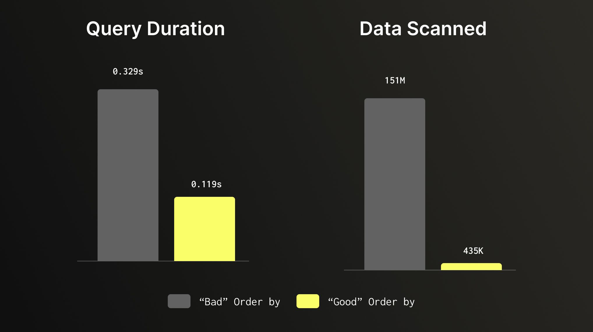
Does a full table scan, reviewing all 150 millions of rows to find a small slice of data. If we use a table with ORDER BY that is set to (product_category, review_date), our query filters based on those columns and makes the same query run 3x faster while scanning 347x less data. Same query, same dataset, that aligns to our query pattern can make a huge difference.
2. Use Efficient Data Types #
Data types in ClickHouse aren't just about correctness, they directly impact storage size, compression ratios, and query speed. Choosing the smallest type that fits your data, avoiding Nullable unless nulls are genuinely meaningful, using LowCardinality(String) for low-cardinality text columns, and preferring Enum over free-text strings for fixed value sets can meaningfully improve both performance and storage efficiency. The same logic applies to integers, using UInt8 or UInt32 instead of UInt64 when your range allows it means less data to read, decompress, and process on every query.
Columns marked as Nullable require ClickHouse to store a separate UInt8 column to track null values, adding overhead to both storage and query execution. So unless nulls are genuinely meaningful, it’s better to avoid using them. In most cases a sensible default can be a viable replacement: an empty string for text fields, 0 for numeric counts, or a sentinel value like -1 for IDs where zero is a valid entry. For string columns with a bounded set of values, LowCardinality(String) uses dictionary encoding under the hood, making it far more efficient for columns with fewer than ~10,000 distinct values.
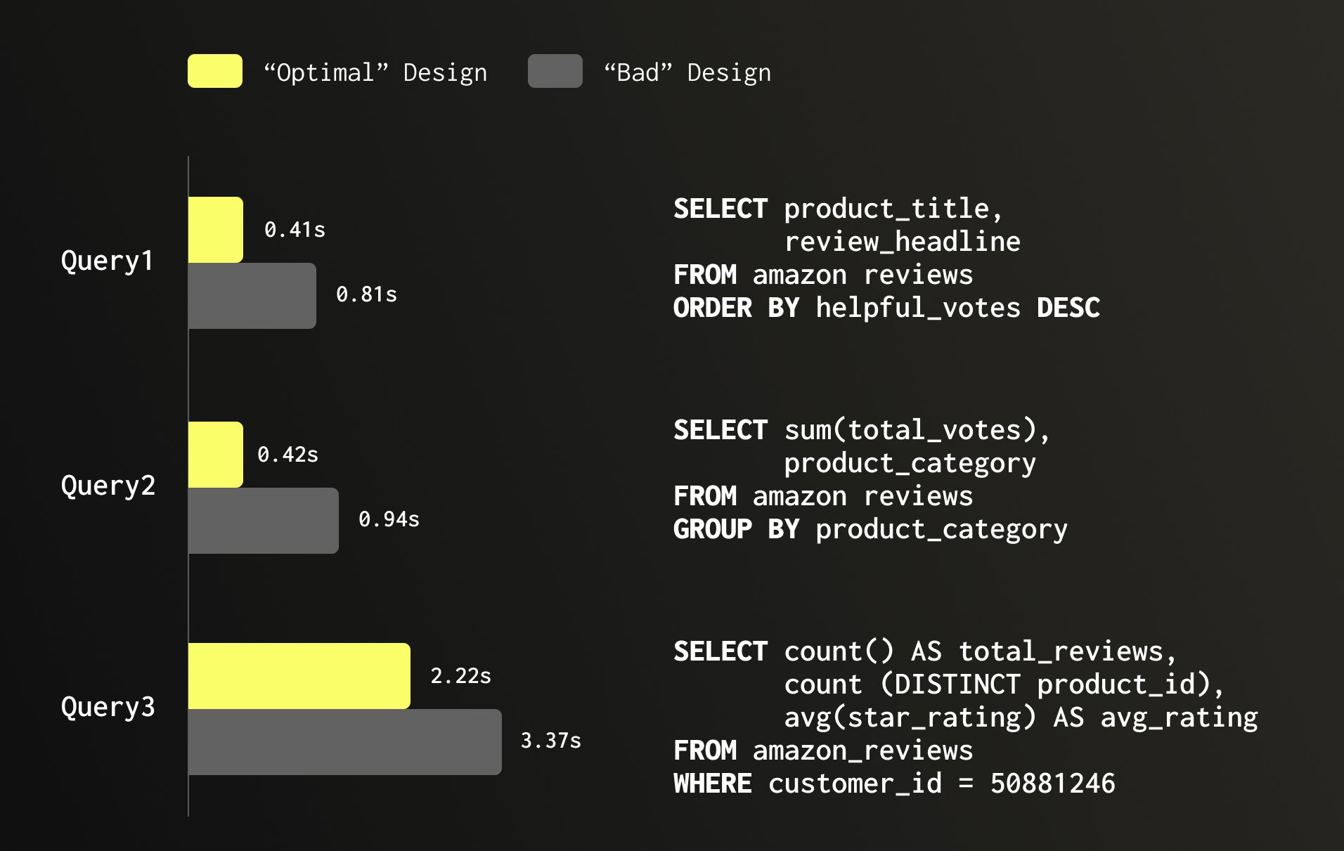
Let’s continue with the Amazon reviews dataset as an example which has 150 million rows. A table which is poorly designed and many columns are Nullable, numeric fields are oversized, and low-cardinality text columns are plain String occupies 30.16 GB. Optimizing it and switching to more aligned data types by dropping Nullable, right-sizing numeric columns, and applying LowCardinality(String) where appropriate, brings storage down to 26.8 GB. But the value is not only on storage, it also has significant improvement on performance as can be seen in the below example, speeding queries making them 2x faster.
3. Consider Your Partitioning strategy, or avoid one #
Partitioning is one of the most misunderstood features in ClickHouse, and the most common mistake is using it as a performance optimization. Partitioning in ClickHouse is primarily a data management feature, not a general-purpose performance accelerator. ClickHouse is already extremely fast at skipping data through primary index pruning. Partitioning on top of that rarely helps and often hurts. The reason is that ClickHouse needs large parts (up to 150GB, often times billions of rows) to compress and query efficiently, and parts never merge across partition boundaries. Over-partitioning such as by day or by a high-cardinality column such as tenant_id often leads to a large number of small parts, slower merges, higher memory usage, and degraded query performance. A good rule of thumb: if you're creating more than a few dozen partitions, you're likely over-partitioning.
So when should you partition? There are two cases when it’s valuable to partition your data. The first is TTL-based data expiration, partitioning by month or year makes it efficient to drop entire partitions of old data without triggering a mutation or merge, which is far more efficient than row-level TTL for large datasets. The second is with merge-oriented table engines like ReplacingMergeTree, CollapsingMergeTree, or AggregatingMergeTree, where we can have significant gains for queries with FINAL by having one part for historical partitions.
Outside of these two scenarios, think carefully before adding a PARTITION BY clause. The default, no partitioning, or a simple partition by month or year is often the right choice.
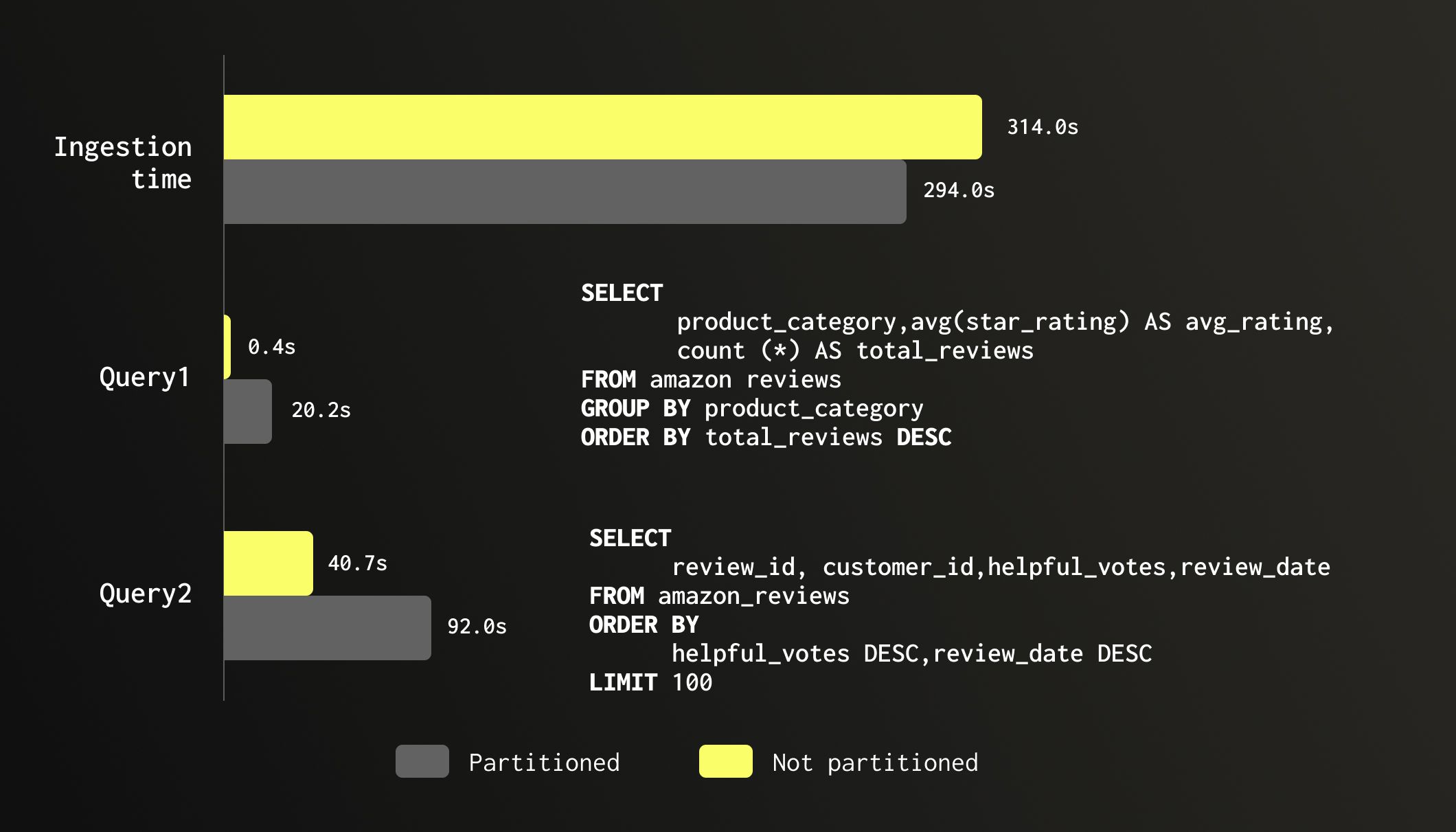
To illustrate the cost of unnecessary partitioning, we tested the same 150 million row Amazon reviews dataset on two identical tables: one partitioned by month of review_date and one unpartitioned. Ingestion time was roughly the same (294s vs 314s), though the partitioned table consumed 55% more memory during load (4.71 GB vs 3.03 GB). The real damage shows up at query time. A simple aggregation across all product_category values ran in 0.4 seconds on the unpartitioned table and 20 seconds on the partitioned one, a 46x slowdown despite scanning the exact same number of rows. A top-100 sort by helpful_votes showed a similar although less significant story: 40 seconds unpartitioned vs 92 seconds partitioned. Same data, same query, twice as slow. The partitioning offered no pruning benefit since neither query filtered on review_date, while the fragmented parts added merge and scheduling overhead on every scan.
4. Optimize Data Scans with Skipping Indexes #
ClickHouse's primary index is a sparse index on your ORDER BY columns and is your most powerful tool for fast data access. But in practice, your queries don't always filter on primary key columns, and when they don't, skipping indexes allows you to extend that same granule-pruning capability to any other column in your schema. Skipping indexes are secondary indexes stored alongside your data without changing how your data is stored and sorted.
There are several types, and it helps to think of them in two buckets: lightweight and heavyweight. Lightweight indexes have minimal impact on write performance and storage, so you can add them freely wherever they'd help. Heavyweight indexes carry higher costs in terms of storage overhead and write amplification, so they're worth adding only when the query acceleration clearly justifies the tradeoff.
Lightweight indexes:
minmax- stores the min and max value per granule. Best for numeric or date columns but can also be useful for strings. Extremely cheap to build and maintain, with negligible storage overhead.set- stores a small set of distinct values per granule. Best for low-cardinality columns you filter on frequently but that aren't part of yourORDER BY. Useset(0)to store all distinct values, or cap withset(N)to fall back to a full scan when exceeded.
Heavyweight indexes:
bloom_filter- a probabilistic structure that answers "is this value definitely not in this granule?". Best for high-cardinality string columns like IDs or URLs. Accepts false positives but never false negatives. Adds meaningful storage and write overhead, so only add it where the scan reduction justifies the cost.ngrambf_v1/tokenbf_v1- bloom filter variants optimized forLIKEorhasTokenqueries on free-text columns. Powerful for substring and token search but expensive to build and store - use them only on columns you actively search on.Text- a new (GA from version 26.2) full inverted index for text search, similar to what you'd find in systems such as Lucene/Elasticsearch. Supports exact term, prefix, and substring matches with high precision. The most powerful option for text search scenarios, but also the heaviest in terms of storage and write amplification. Use it whenBloom_filteris not fast enough for your needs.
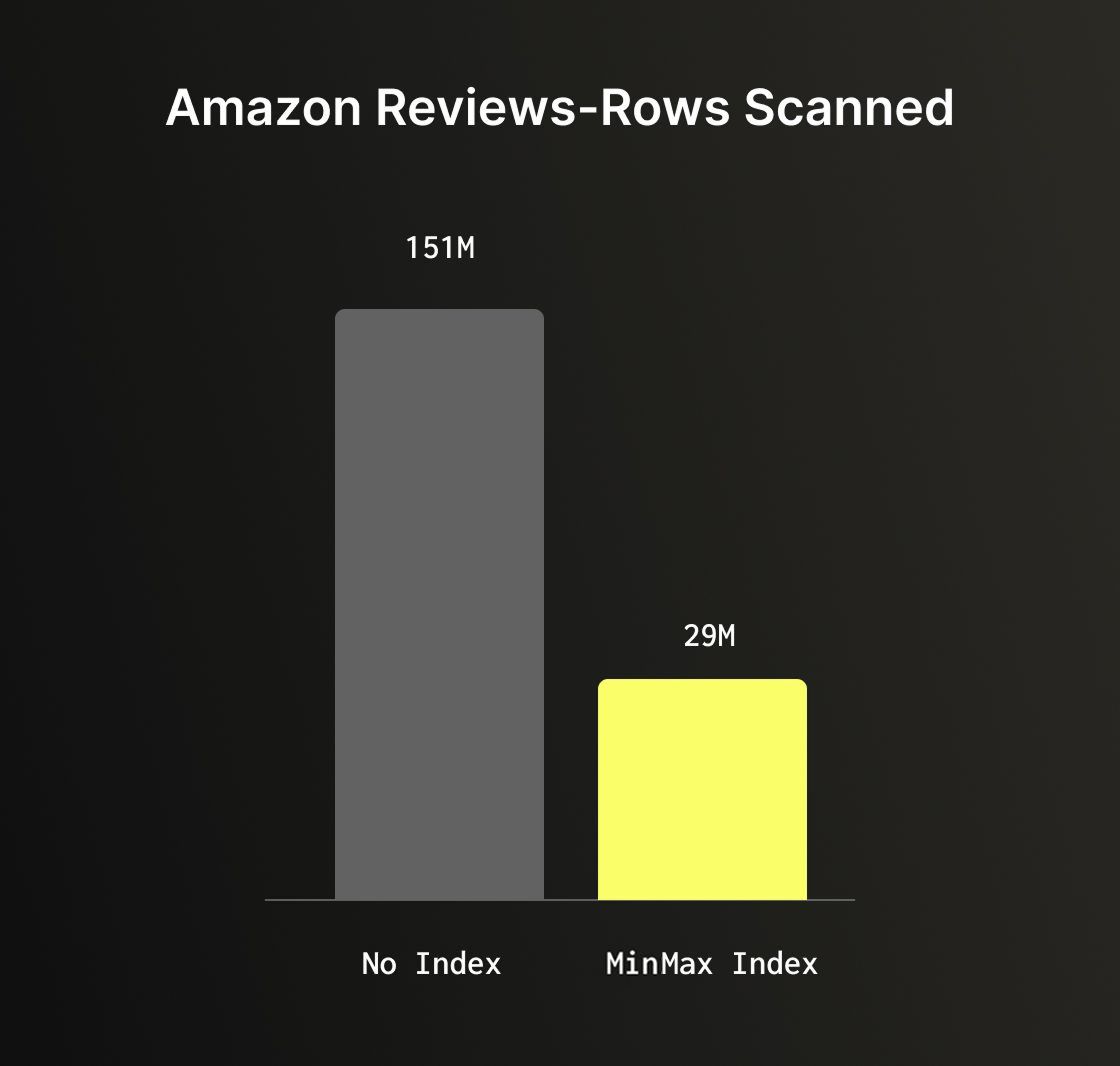
The Amazon reviews dataset can help illustrate the benefit of skipping indexes well. A query filtering on total_votes > 1000 with no skipping index performs a full table scan of all 150 million rows. Adding a minmax index on the total_votes column, one of the cheapest indexes you can add, reduces scanned rows to just 29 million, an 80% reduction with very minimal to no overhead.
5. Leveraging the JSON Data Type for semi-structured data #
ClickHouse's native JSON type is a powerful tool for handling semi-structured data where keys are unpredictable, change over time, or carry values of varying types. It automatically infers types at insert time and stores each discovered path as a separate subcolumn (up to the max_dynamic_paths defined), giving you columnar performance on dynamic data.
However this flexibility comes with trade-offs. The JSON type performs type inference on every insert, which adds overhead compared to a static schema. It also consumes more storage when paths contain values of more than one type. For data with a known, consistent structure, even if it arrives in JSON format a static schema with explicit column types will always outperform it.
A key parameter to understand when using JSONs is max_dynamic_paths, which controls how many distinct JSON paths ClickHouse will store as individual subcolumns. By default once that limit is exceeded, additional paths are stored together in a single shared structure, which is less efficient to query. The default is 1024, but for payloads with a bounded and well-known set of paths, setting it lower keeps things tighter and more predictable. When you know that certain paths will always be present and always carry the same type, you can use JSON hints to declare them explicitly. For example:
1CREATE TABLE events (
2  id UInt64,
3  payload JSON(`timestamp` DateTime, `level` LowCardinality(String))
4)
5ENGINE = MergeTree
6ORDER BY id;
Hints provide ClickHouse more information about those paths, they're stored and compressed like regular columns while the rest of the payload remains fully dynamic.
When converting Amazon Reviews dataset to a document based dataset, using hints reduced storage by 38% vs JSON without hints and this example query was 26% faster when using hints vs. without ones.
1SELECT count(*),
2       review_data.product_category PC
3FROM   amazon_reviews_json
4GROUP  BY pc
However this is not only for storage and improving performance, hinted paths are also reliable targets for skipping indexes, whereas fully dynamic paths can be inconsistent across granules and yield lower index effectiveness. It's important to call out that you can add a skipping index on any JSON path, but casting would be required.
The bottom line: if data is flat with predictable structure, use explicit columns. If it has a predictable core with dynamic variations, consider using static columns for the known parts and a single JSON column for the rest. Reserve a fully dynamic JSON column for cases where the schema is genuinely unpredictable.
6. Getting data into ClickHouse the right way #
Inserting data into ClickHouse efficiently is an important topic to consider. There are four common ingestion patterns, and each has a recommended approach and best practices.
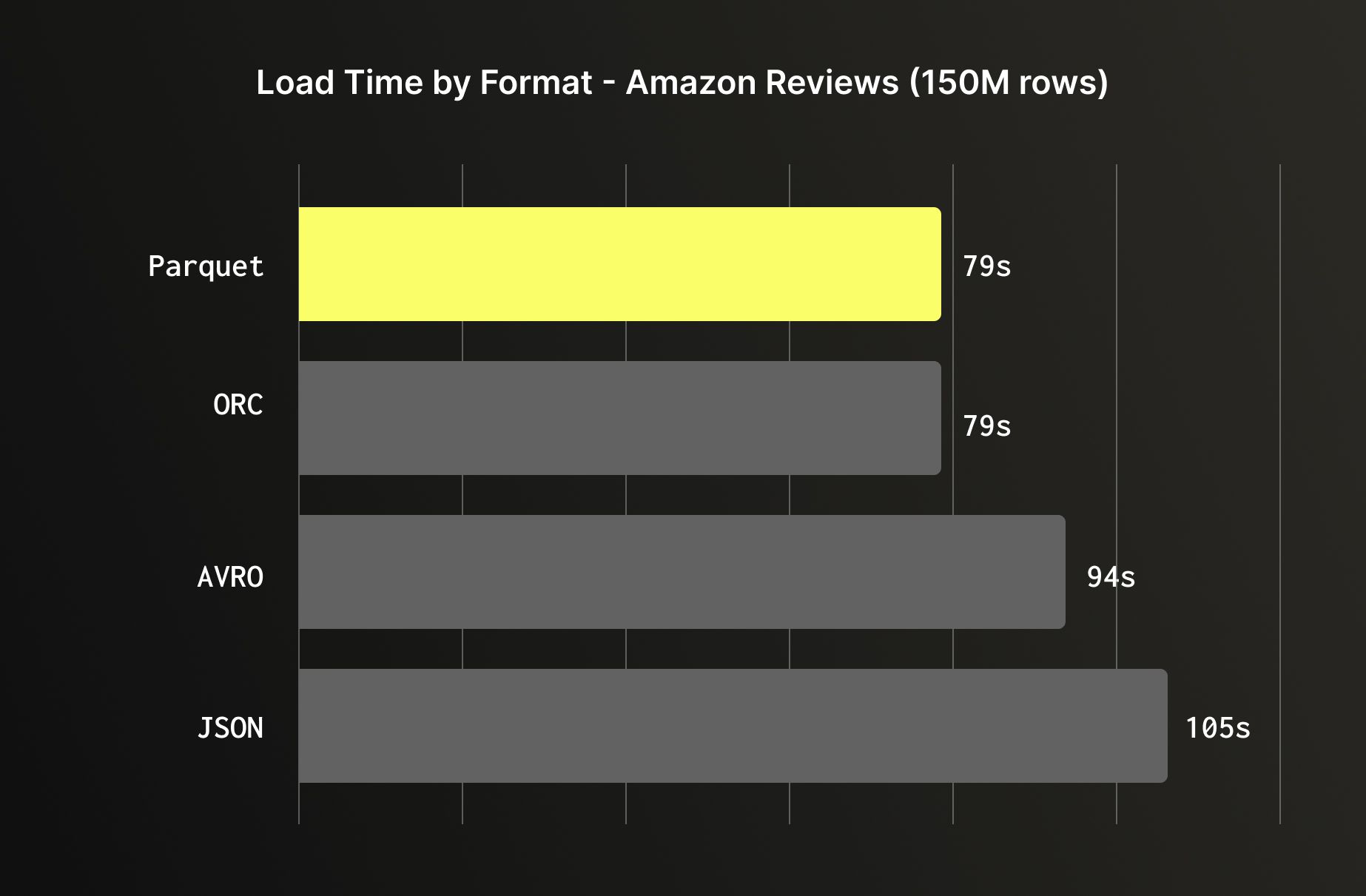
Object storage (Amazon S3, GCS, Azure Blob) is one of the most common sources for bulk loading. When you have a choice of format, prefer columnar formats like Parquet or ORC over row-based ones like JSON or Avro; ClickHouse can read only the columns it needs from Parquet and ORC, skipping the rest entirely, while JSON requires parsing every field on every row. But even when loading all columns, columnar formats are still faster as the data arrives already organized the way ClickHouse stores it internally, reducing the conversion overhead during ingestion. Loading the Amazon reviews dataset illustrates this clearly: Parquet and ORC loaded in 79 seconds, Avro in 94 seconds, and JSON in 105 seconds.
For managed, ongoing ingestion from object storage, ClickPipes supports S3 and GCS sources directly.
CDC from databases (Postgres, MySQL, MongoDB, etc) and event streams (Kafka, Kinesis, etc) are best handled through ClickPipes, ClickHouse Cloud's native managed ingestion service. ClickPipes handles schema mapping, offset management, error handling, and backpressure out of the box. For CDC specifically, it uses a log-based approach that captures every row-level change with minimal load on the source database. If your database lives in a private VPC, ClickPipes supports reverse PrivateLink, allowing secure connectivity without exposing your database to the public internet.
Backend applications writing directly to ClickHouse is a very common way companies use, however it does require taking into account a few considerations. ClickHouse is optimized for large, infrequent batches, not the small, frequent inserts typical of application code. Each insert creates at least one part in the storage layer, and too many small parts lead to merge pressure, elevated memory usage, and eventual insert throttling. The two solutions are batching on the client side (accumulate rows and flush every few seconds or a few thousand rows), or enabling async inserts, which lets ClickHouse buffer incoming inserts and flush them in batches automatically:
1SET async_insert = 1;
2SET wait_for_async_insert = 1;
With wait_for_async_insert = 1, the client waits for confirmation that the data has been flushed to a part providing you the convenience of small writes with proper acknowledgement and reliable error handling. You can monitor async insert behavior via system.asynchronous_insert_log to tune flush intervals and buffer sizes for your workload.
Regardless of the ingestion method: avoid inserting one row at a time, prefer native binary formats over JSON where possible, and monitor part counts in system.parts to identify ingestion problems early.
7. Compute on write, faster reads with materialized views and projections #
Both materialized views and projections follow the same core idea: do work at insert time so that reads are faster and less compute heavy. Instead of scanning and aggregating at query time, you pre-compute and store results as data arrives. The tradeoff is the same for both: faster reads come at the cost of increased storage and additional write overhead.
Projections are alternative sort orders or pre-aggregations stored physically inside the same table. When ClickHouse executes a query, it automatically selects the best projection if one matches the query's filter and sort pattern so no query changes are required. This makes them transparent to the application and easy to adopt. The downside is that every insert must write and sort data for each projection, increasing both insert latency and storage footprint. Before building a query optimization strategy around projections, it's worth validating that they're actually being selected at query time. The easiest way is to use:
1SET force_optimize_projection = 1;
With this setting enabled, ClickHouse will throw an error if no suitable projection is found for your query making it immediately clear whether your projection is being used or silently ignored.
An important callout on projections is that they are oftentimes being added "just in case" and impacts storage and insert costs. It’s important to first use a well-designed primary key and identify queries that are actually slow, then add projections only where they're needed. Let real usage data guide projection definitions.
Materialized views have two flavors. Refreshable materialized views work like you'd expect from a traditional data warehouse, they recompute the result on a schedule, making them suitable for complex transformations but oftentimes requiring you to manage bookmarks, understanding what was processed already vs what hasn’t, require reprocessing in cases of late arrivals or backfills to historical data and strongly recommended to handle taking into consideration idempotency. Incremental materialized views are more unique to ClickHouse and more flexible but require more deliberate design. They act as insert triggers, running a SELECT on each incoming batch and writing the result to a target table which makes them extremely efficient for continuously maintaining aggregations, summaries, or fan-out pipelines as data arrives. The important constraint is that they are only triggered on inserts: deletes and updates to the source table are not propagated, so they're best suited for append-only or immutable data patterns.
Joins inside incremental materialized views deserve special attention as only the left-hand table in the join triggers the view. If the right-hand side changes, the materialized view won't update. It's also worth knowing that materialized views compose well: a single source table can fan out to multiple MVs, each maintaining a different aggregation or transformation, and multiple MVs from different source tables can feed into the same destination table, making them a powerful building block for more complex data pipelines.
A common pattern in ClickHouse is to use materialized views to maintain pre-aggregated summary tables for dashboards and high-frequency queries, while keeping the raw table for ad-hoc exploration.
8. Know your system tables #
ClickHouse's system tables are one of its most powerful built-in features. Everything happening inside your cluster: queries, merges, background activity, errors, it is all captured and queryable with standard SQL, giving you deep observability using standard SQL.
On a multi replica service, querying system tables only shows you the logs from the replica your query runs against. To get a full picture across all replicas, use clusterAllReplicas. And since many system tables rotate, historical data might not show up unless you explicitly merge across them using the merge table function. Here is an example of how to query system.query_log to ensure you get all service logs for the table:
1SELECT event_time, query_id, query, type
2FROM   clusterAllReplicas('default', merge('system', '^query_log*'))
3WHERE  event_time > Now() - toIntervalMinute(5);
2 of the most useful system tables to get familiar with are system.query_log and system.parts.
system.query_log is a primary tool for understanding query behavior. Every query generates one row per event: QueryStart, QueryFinish, ExceptionBeforeStart, or ExceptionWhileProcessing providing a complete lifecycle view of every query that runs on the service. Each row captures timing (query_duration_ms), resource usage (read_rows, read_bytes, memory_usage), the query text itself, and which databases, tables, columns, and projections were involved. For error investigation, exception_code, exception, and stack_trace are available. The ProfileEvents column goes deeper, it's a map of low-level execution counters that can reveal exactly where time is being spent, from CPU cycles to I/O reads to cache hits. When a query is slower than expected, ProfileEvents often tells whether the bottleneck is I/O, CPU or network.
system.parts exposes detailed information about every physical data part in your storage for all MergeTree-family tables. Each row corresponds to one part, making it the go-to table for monitoring storage, diagnosing merge behavior, and understanding the health of tables. The most important columns to know are: active tells whether a part is currently live or a leftover from a completed merge so filtering on active = 1 keeps queries focused on relevant parts. partition and partition_id show which partition each part belongs to, while rows, bytes_on_disk, data_compressed_bytes, and data_uncompressed_bytes give a clear picture of size and compression efficiency. part_type distinguishes between Wide and Compact parts, which affects how columns are stored. In Wide format, each column is stored in its own separate file, this is the standard format for larger parts and enables efficient column pruning at read time. Compact format stores all columns in a single file (by default less than 10MB), which reduces the number of file handles and is more efficient for small parts with few rows.
2 queries that can be valuable to keep handy are:
Part count and size per table:
1SELECT table, count() AS parts, sum(rows) AS total_rows,
2       formatReadableSize(sum(bytes_on_disk)) AS size_on_disk
3FROM   system.parts
4WHERE  active
5GROUP  BY table
6ORDER  BY parts DESC;
Over-partitioned tables:
1SELECT table, partition, count() AS parts
2FROM   system.parts
3WHERE  active
4GROUP  BY table, partition
5HAVING parts > 10
6ORDER  BY parts DESC;
9. Perfecting ReplacingMergeTree #
ReplacingMergeTree is one of the more popular table engines, it is used for supporting use-cases in which you need to support deduplication or upserts. This table engine keeps the latest version of each row based on a defined column (e.g. version/timestamp). The deduplication takes place based on the uniqueness of the defined ORDER BY columns. The discarding of older duplicates occurs during background merges. The thing to remember is that these merges happen asynchronously, meaning duplicate rows can exist at query time. Getting correct results requires either the use of FINAL or the argMax pattern, and understanding the tradeoff between them.
FINAL is the simplest approach, adding it to the query and ClickHouse handles deduplication transparently. The cost is that FINAL must reconcile all parts before returning results, and its performance is directly tied to how many parts exist at query time. On a well-merged table with a single part in a partition, FINAL would be just as fast as not using FINAL. On a table mid-ingestion with many parts, it can carry a significant overhead.
1SELECT star_rating
2FROM   mytests.amazon_reviews_rmt FINAL
3WHERE  review_id = ''
The argMax pattern is an alternative that folds deduplication into the aggregation itself, picking the value from the row with the highest version:
1SELECT argMax(star_rating, review_date)
2FROM   mytests.amazon_reviews_rmt
3WHERE  review_id = ''
On the Amazon reviews dataset with 152 million rows (150M originals + 2M duplicates), the difference between the two approaches depends heavily on table state. With 9 unmerged parts, the above query using FINAL took 1.5 seconds vs argMax at 1.0 seconds.
To demonstrate the difference with fewer parts, we forced the parts to consolidate to a single part, both dropped to roughly the same level: 0.48s vs 0.40s. Results can vary depending on query shape, cardinality, and part count, but the pattern holds: argMax tends to be more consistent regardless of merge state, while FINAL improves significantly as parts consolidate.
In practice, FINAL is a simpler choice for queries or when the table is well-merged. argMax is worth reaching for when you need predictable latency on a table receiving active inserts.
One way to reduce the variability of FINAL in production is to configure background merges to be more aggressive on older data. By default, ClickHouse merges parts based on internal heuristics which factors part size, count, and age but has no obligation to ever consolidate a partition down to a single part. This means a table can sit indefinitely with multiple parts per partition, keeping FINAL overhead. The min_age_to_force_merge_seconds setting changes this behavior by forcing ClickHouse to keep merging parts older than the specified threshold until only one part per partition remains:
1min_age_to_force_merge_seconds = 600,
2min_age_to_force_merge_on_partition_only = 1;
Keep in mind that this can increase background merge workload as ClickHouse will continuously merge parts until each partition has only one, consuming more CPU and I/O that could otherwise be used for queries or inserts.
The min_age_to_force_merge_on_partition_only = 1 flag ensures this only triggers on partitions where all parts are old enough, avoiding interference with partitions still actively receiving writes. It’s important to call out that for this setting to be effective in practice, tables should be partitioned. Without partitioning, all data lives in a single partition that can accumulate too much data. Since ClickHouse by default won't merge parts that would result in a part exceeding 150GB, consolidating down to a single part becomes unrealistic. With partitioning by month or year, each partition stays within a manageable size range where merging down to a single part is achievable, which is exactly the state where FINAL performs best.
10. Optimize your joins #
Historically, JOINs in ClickHouse were something users were advised to approach with caution, and the common guidance was to avoid them where possible through denormalization, dictionaries, or materialized views. That advice made sense at the time, but significant engine-level improvements have made JOINs increasingly viable for high-concurrency production workloads. The introduction of the Analyzer (query planner) as the default query execution layer brought major improvements to join planning: ClickHouse 24.4 introduced better predicate pushdown that can deliver 10x query improvements by pushing filter conditions to both sides of a JOIN, version 24.12 gained the ability to automatically reorder two-table joins to place the smaller table on the right-hand side, and 25.9 extended this to queries joining three or more tables. Combined with a wide selection of join algorithms to cover different memory and performance tradeoffs, JOINs in ClickHouse today are meaningfully more capable and easier to use correctly than they were even a year ago.
That said, JOINs still come with a cost in an analytical database, and a few principles are worth following. For real-time workloads where millisecond latency matters, aim for a maximum of 3 to 4 joins per query. In addition, denormalization, dictionaries, or pre-aggregated materialized views are tools worth considering for even faster query performance.
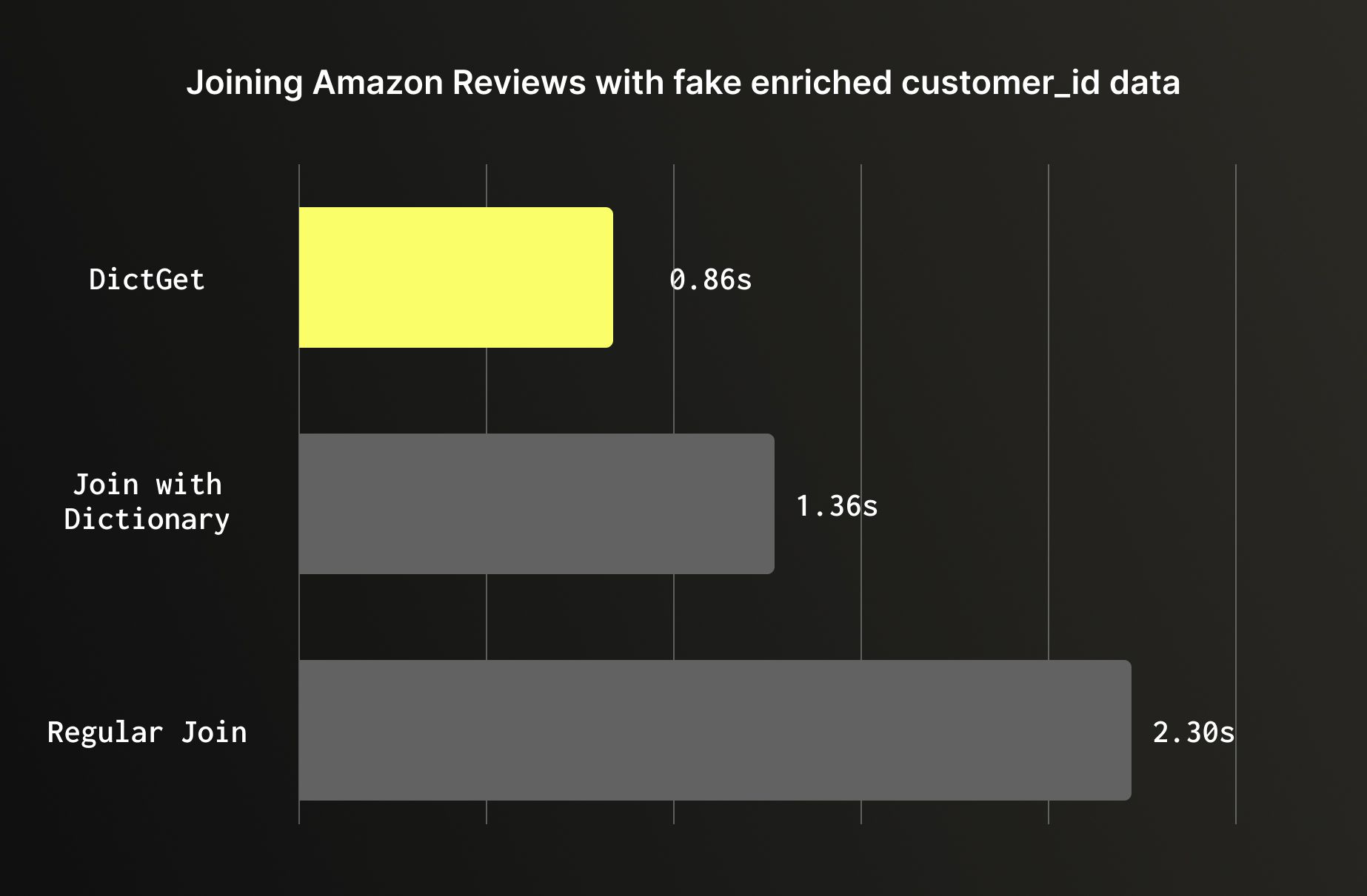
For static or slowly changing lookups it’s recommended to use dictionaries. When enriching a large table with data from a smaller reference table that doesn't change frequently, a dictionary will outperform a regular join. Dictionaries are loaded entirely into memory and accessed via dictGet, bypassing the hash join process entirely. On the Amazon reviews dataset enriched with customer metadata, the difference is significant: a regular JOIN on 150M rows ran in 2.3 seconds, a join against a dictionary table completed 1.36 seconds, and dictGet took 0.86 seconds; Nearly 3x faster than the baseline join, with no change to the underlying data.
Wrapping Up #
ClickHouse is extremely fast out of the box, but getting the most out of it requires understanding how it stores, merges, and queries data. The best practices in this post aren't isolated tips, they build on each other. A well-chosen ORDER BY often makes skipping indexes more effective. Good data types reduce the work that materialized views and projections have to do. Sensible partitioning makes ReplacingMergeTree and TTL-based expiration work cleanly. Getting ingestion right keeps your part counts healthy, which in turn keeps FINAL fast.
The Amazon reviews dataset benchmarks throughout this post illustrate that these aren't marginal gains, the right primary key scans 347x less data, the right data types cut storage by 12% and shorten query time by 50%, unnecessary partitioning can slow queries by 46x, and a dictionary lookup can be 3x faster than a regular join. These are order-of-magnitude differences that come purely from design decisions, not hardware.
If you're just getting started, focus on the first two: primary key design and data types. They have the broadest impact and apply to every table you create. From there, add skipping indexes where your queries need them, partition only when you have a clear reason to, and reach for materialized views and ReplacingMergeTree as your use case demands.
ClickHouse rewards users who understand its architecture. The more your schema and queries align with how ClickHouse manages data, the faster and more efficient your system will be. At its best, that means allowing you to ingest billions of rows and querying them in milliseconds.


