TL;DR
Multi-stage distributed execution gives ClickHouse Cloud a new way to scale one query across many nodes. It repartitions intermediate data between stages, removing key bottlenecks in large joins and high-cardinality aggregations.
Early TPC-H results show up to 3.4× speedups for join-heavy queries while retaining near-linear aggregation scaling: 7.4× faster on 8 nodes than on 1 node.
Scaling one query across many nodes #
ClickHouse has always been able to scale a single query across multiple nodes. In shared-nothing deployments, users do this with physical sharding and the Distributed table engine. In ClickHouse Cloud, parallel replicas brought intra-query scaling to shared storage.
These mechanisms work well for many analytical queries, but they were not the final answer for modern PB-scale workloads. They could fan out work across nodes, but they could not freely repartition intermediate results between execution stages. That limited how far ClickHouse could scale high-cardinality aggregations, and especially large joins.
Multi-stage distributed query execution is the next step. It gives ClickHouse Cloud a new way to parallelize a single query across the CPU and memory of all available nodes, without the bottlenecks of the previous execution models.
In this post, we introduce the new extension of ClickHouse’s query execution model and walk through how it works. We use a multi-table join as the running example because joins are among the hardest analytical workloads to scale, but the mechanism is much broader: it is a new foundation for distributed query execution in ClickHouse Cloud.
Before we look at the new mechanics, let’s review what came before and why those approaches weren’t enough for modern PB-scale workloads.
Why existing distributed execution was not enough #
The existing distributed execution was useful but not elastic enough for PB-scale workloads.
In shared-nothing open source deployments, ClickHouse scales a query by physically sharding data across nodes and querying those shards through a Distributed table. Each node processes its local slice, and the requester merges the results.
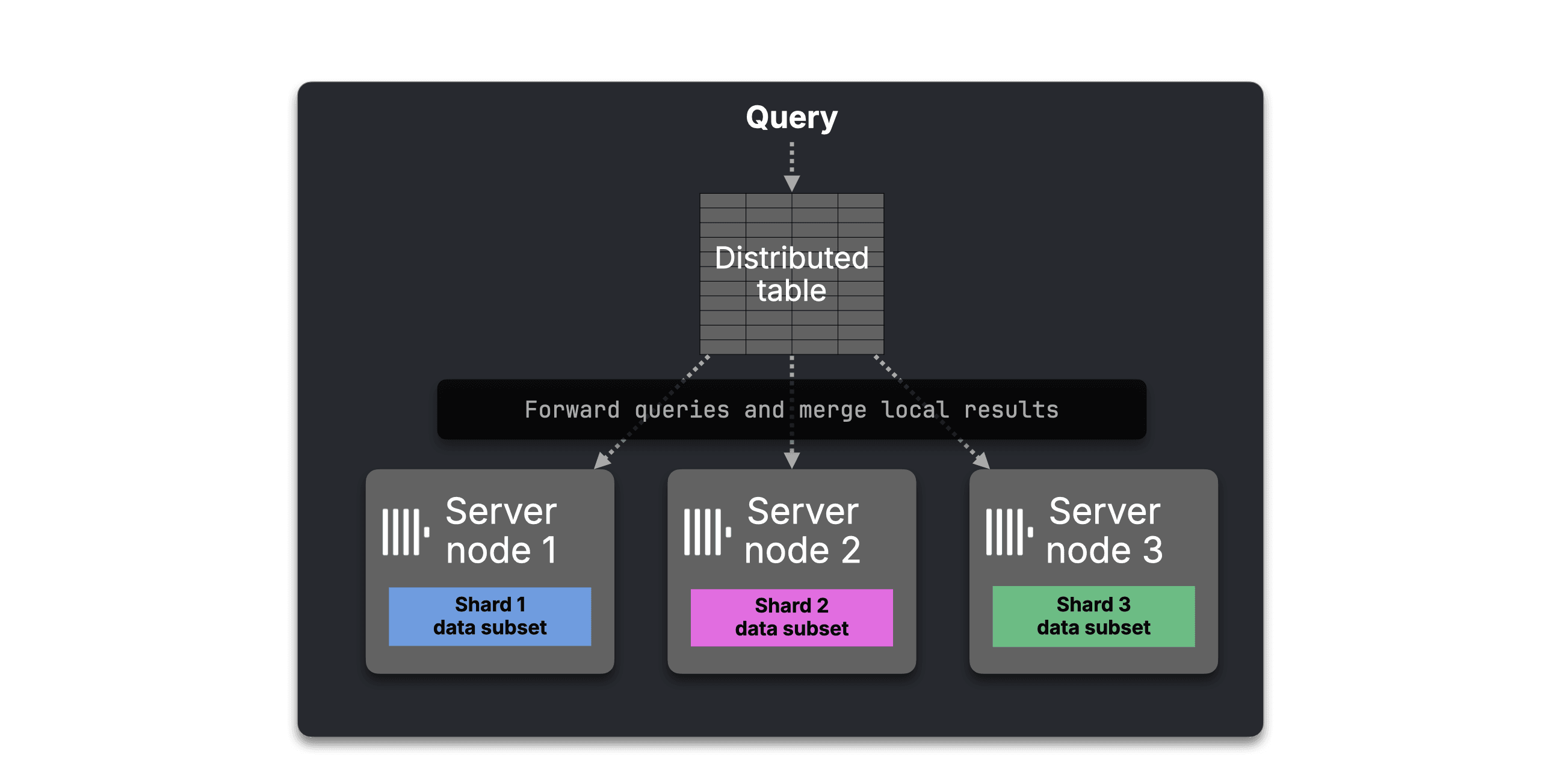
That works, but capacity is tied to the shard layout.
Bottleneck: capacity is tied to shard layout
Adding compute does not automatically make one query faster. Large tables must first be redistributed across more shards.
Large joins across physically sharded tables expose a second limitation. A join only works when matching rows meet on the same machine. With a distributed JOIN, each node keeps its local left side, fetches the missing right-side shards from the other nodes, builds a full right-side hash table, and returns its local join result to the requester.
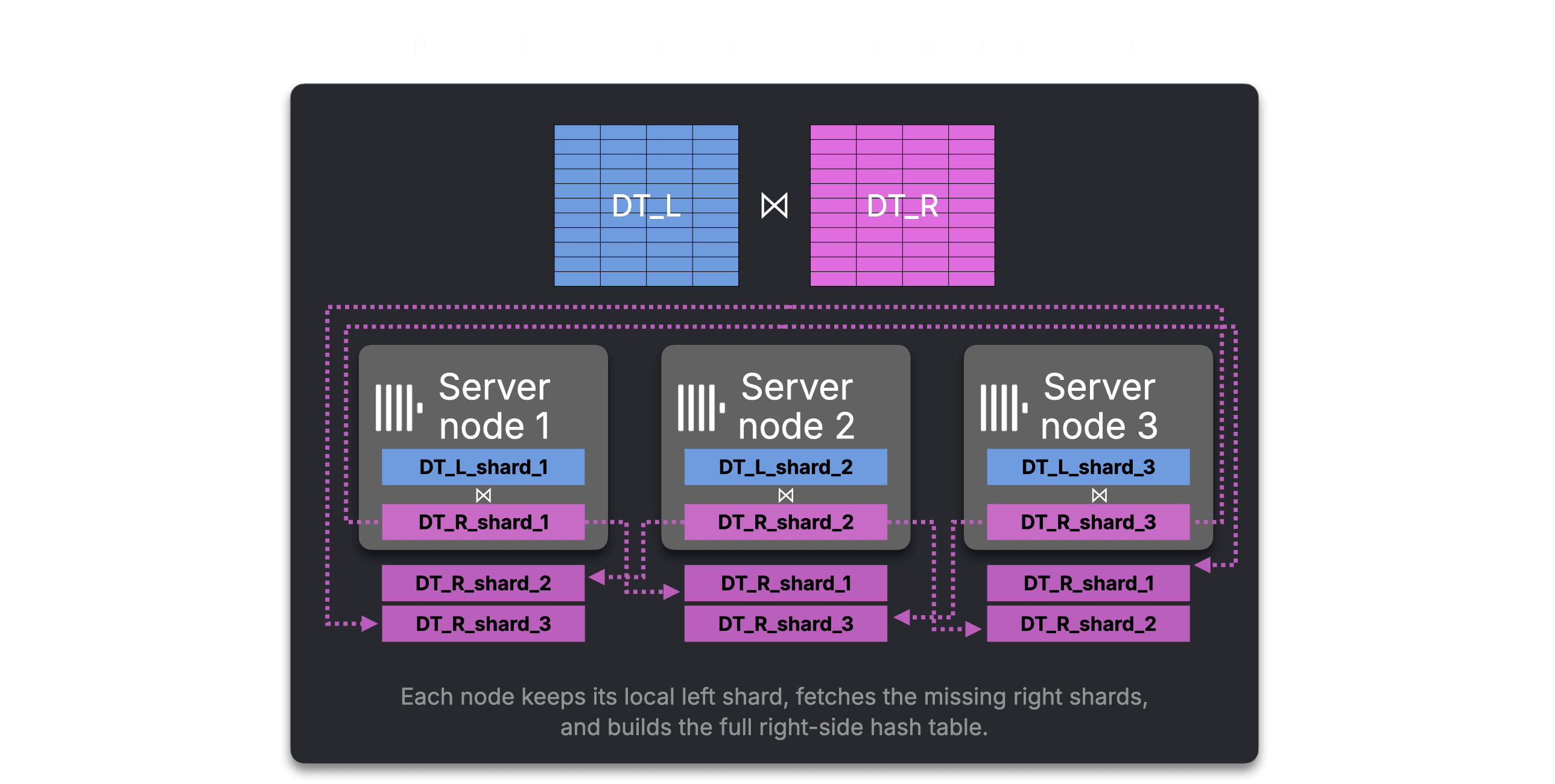
GLOBAL JOIN reduces the many-to-many network round-trip by computing the right side once and broadcasting it to every node.
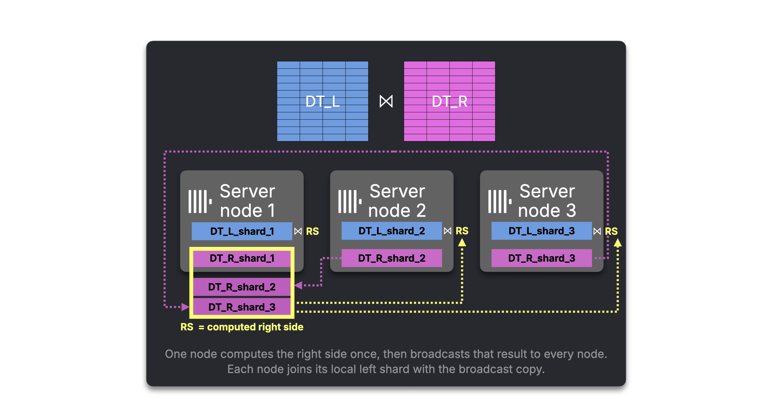
But the core problem remains: large right sides still have to be copied across the cluster.
Bottleneck: large right sides are copied everywhere
Distributed JOIN and GLOBAL JOIN handle network traffic in different ways, but both still make every shard join against a full right side.
ClickHouse Cloud removed the physical sharding problem by moving to shared storage. Any node can access the same table data, and parallel replicas allow multiple nodes to participate in a single query. Nodes can be added or removed instantly, with no data copying or reshuffling.
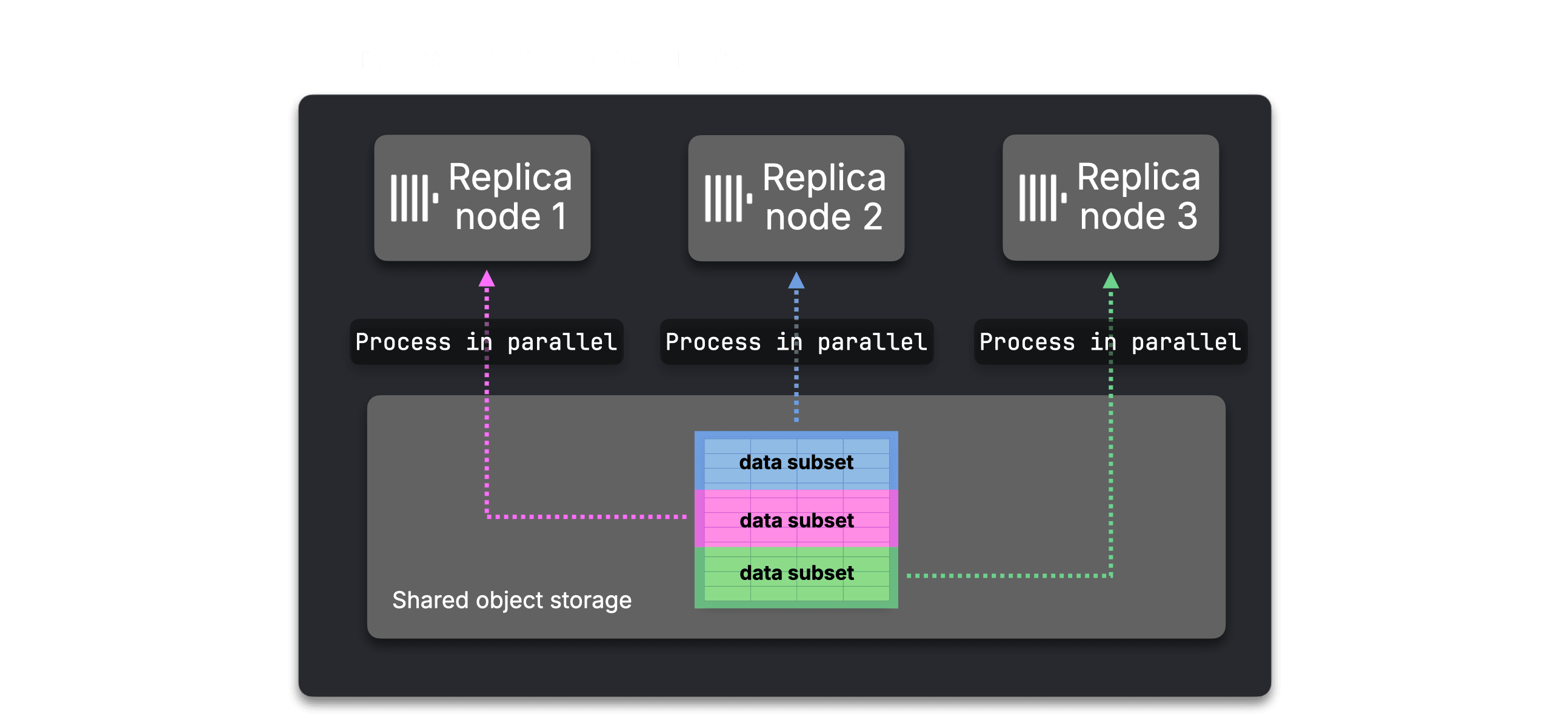
That made intra-query scaling in ClickHouse Cloud much more elastic. But parallel replicas still had a structural limitation: they could split work across replicas, but they could not freely repartition intermediate data between execution stages.
This shows up in two places.
First, joins. On a single node, ClickHouse can parallelize both sides of its default hash join strategy: it partitions rows by the join key into multiple hash tables, so both build and probe work can run across CPU cores. The same remains true inside each node when parallel replicas are used.
The limitation is one level higher. Across multiple nodes, dividing the build side itself would require a shuffle stage that repartitions both inputs by join key between nodes. Parallel replicas do not have that mechanism. The next best option is to distribute the left-side read ranges after primary-index pruning. That parallelizes probe-side work across nodes, but those ranges are not partitioned by the join key. A row in one left-side range can match rows anywhere in the right-side table, so each node still needs the full right side to build its local hash table(s) before probing its local slice.
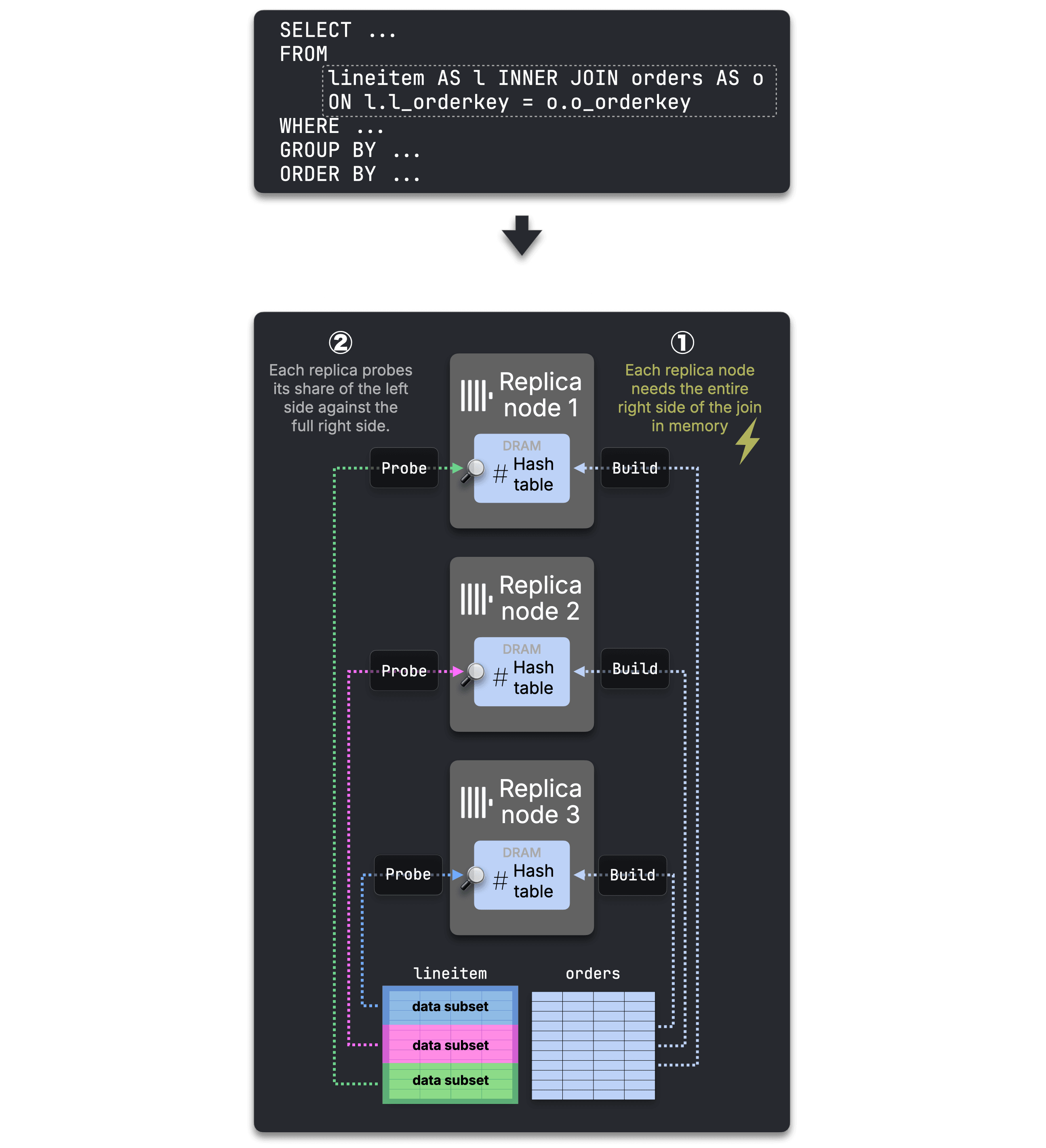
Bottleneck: the build side does not scale out
The left-side probe is divided across nodes, but the build side is not. Every node still builds the same hash table from the full right side, so the build step is repeated instead of divided across the cluster.
Second, aggregations. Nodes can scan and aggregate locally in parallel. But without a shuffle by the GROUP BY key, ClickHouse cannot guarantee that all rows for the same GROUP BY key end up on the same node.
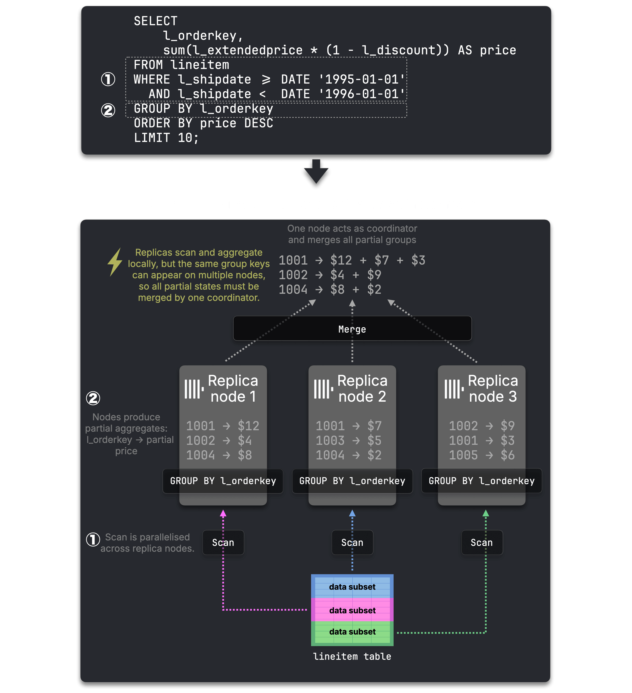
Bottleneck: final aggregation is still single-node
Partial groups must be merged by one coordinator. For high-cardinality GROUP BY, that final merge is bounded by one node’s CPU and memory, not the cluster.
Both problems have the same root cause: there is no general way to repartition intermediate data between execution stages. That is what multi-stage distributed execution adds.
Introducing multi-stage distributed execution #
Multi-stage distributed execution adds the missing primitive: it lets ClickHouse Cloud move intermediate data between nodes while a query is running.
Instead of executing a query as one distributed fan-out plus a final merge, ClickHouse splits the query plan into stages running in parallel across worker nodes. Between stages, exchange operators move the intermediate results into the shape required by the next stage.
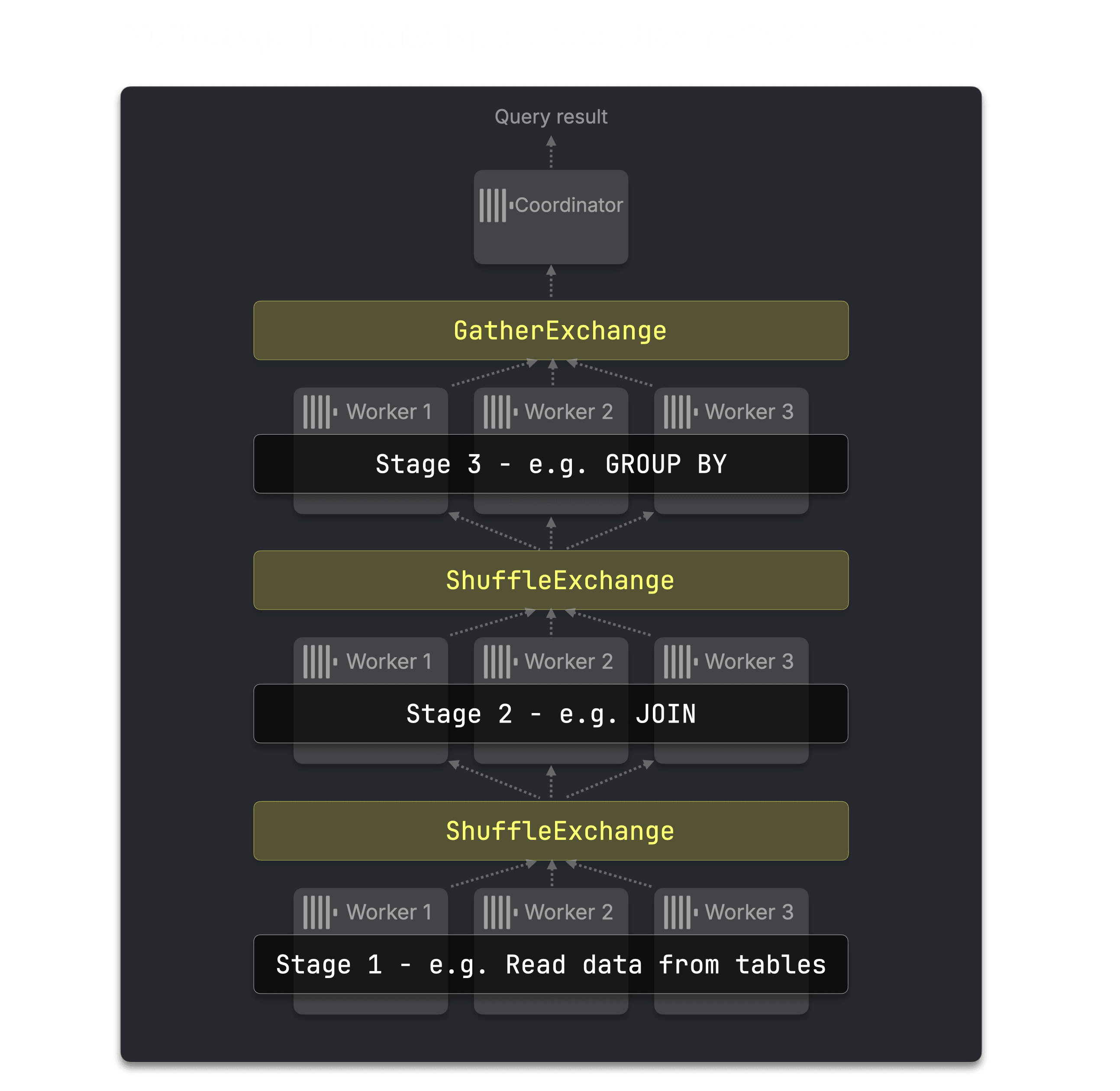
For example, data can be shuffled by a join key so each worker receives the matching slice of both join inputs. It can be shuffled by a GROUP BY key so each worker owns complete groups. Small inputs can be broadcast to all workers. Final results can be gathered by the coordinator.
Prior bottlenecks removed: data can move between stages
Large joins no longer need every node to build the full right-side hash table. High-cardinality aggregations no longer need one coordinator to merge all partial groups.
The core abstraction is the exchange operator, a well-known building block in parallel query execution, introduced for the Volcano system and used by MPP databases like Teradata and Greenplum, as well as in SQL Server.
The exchange operator redistributes data between plan stages. Multi-stage distributed execution uses three main exchange types:
-
GatherExchange (N-to-1): sends worker output to the coordinator, usually at the top of the plan to produce the final result.
-
ShuffleExchange (M-to-N): repartitions rows by a key, such as a join key or GROUP BY key. This is what lets each worker own a complete, disjoint slice of the next operation.
-
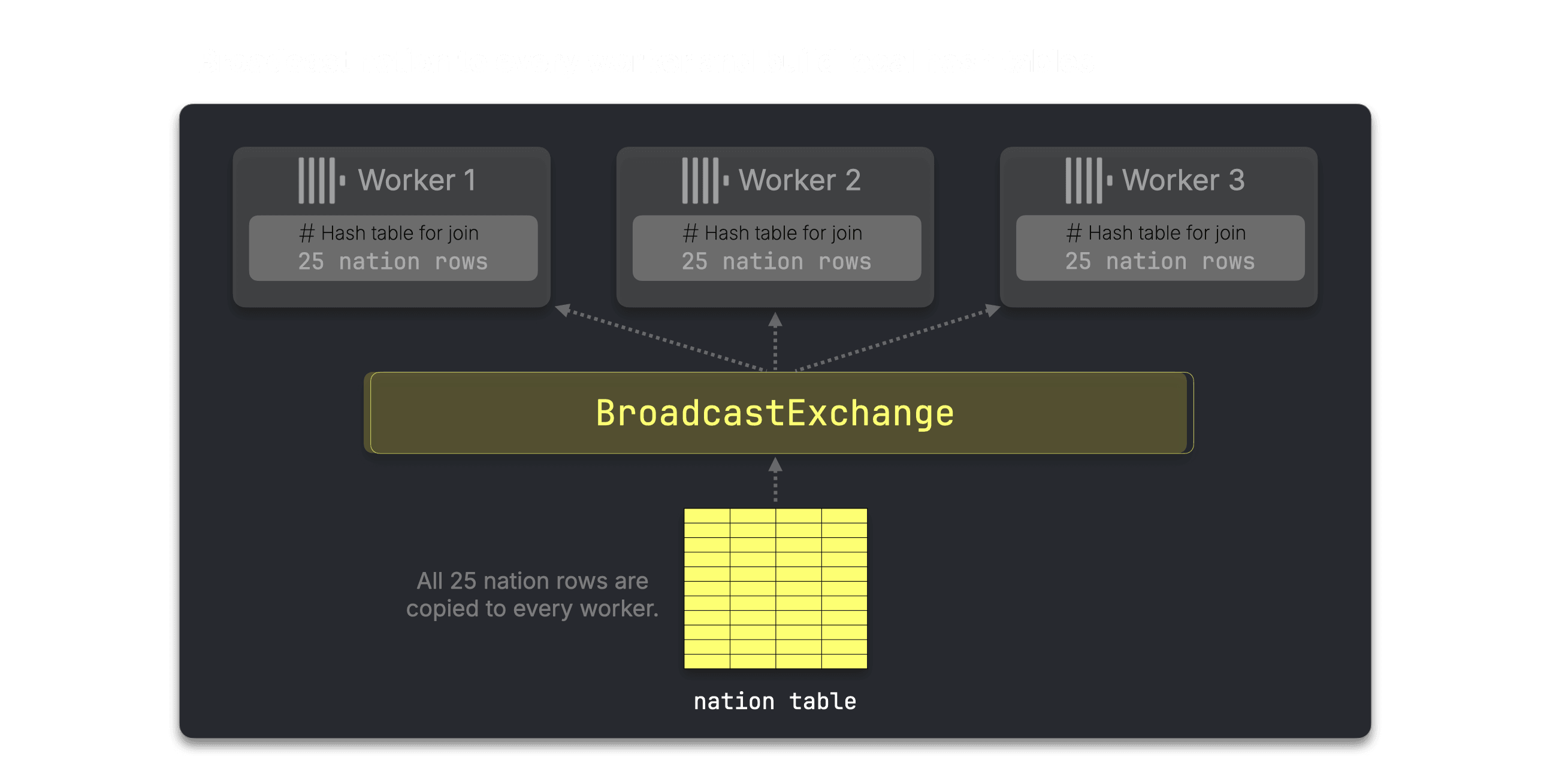
BroadcastExchange (1-to-N): copies a small input to every worker, useful when one side of a join is small enough to replicate cheaply.
There is also ScatterExchange, which spreads rows randomly amongst workers.
Those are the mechanics in the abstract. The easiest way to see why they matter is to follow one query through the stages.
How one analytical join query avoids the old bottlenecks #
Let’s make this concrete with a TPC-H-like query that hits both bottlenecks from the previous section: a large join side that should not be copied to every worker node, and an aggregation that should not collapse into a single-node final merge.
The query computes total shipment revenue per nation: it joins lineitem to supplier, joins the result to the small nation table, groups by n_name, and sorts by revenue.
SELECT n_name, sum(l_extendedprice) AS revenue
FROM lineitem
JOIN supplier ON l_suppkey = s_suppkey
JOIN nation ON s_nationkey = n_nationkey
WHERE l_shipdate >= '1994-01-01' AND l_shipdate < '1995-01-01'
GROUP BY n_name
ORDER BY revenue DESC;
The distributed plan (inspected via EXPLAIN) contains one BroadcastExchange, two ShuffleExchanges, and one GatherExchange:
┌─explain──────────────────────────────────────────────────┐
│ Output: n_name, sum(l_extendedprice)                     │
│                                                          │
│ GatherExchange (sorted by (sum(l_extendedprice) DESC))   │
│ └──Sorting (Sorting for ORDER BY)                        │
│    └──Aggregating                                        │
│       └──ShuffleExchange (by hash([n_name]))             │
│          └──JoinLogical                                  │
│             ├──ShuffleExchange (by hash([l_suppkey]))    │
│             │  └──ReadFromMergeTree (sf100.lineitem)     │
│             └──ShuffleExchange (by hash([s_suppkey]))    │
│                └──JoinLogical                            │
│                   ├──ReadFromMergeTree (sf100.supplier)  │
│                   └──BroadcastExchange                   │
│                      └──ReadFromMergeTree (sf100.nation) │
└──────────────────────────────────────────────────────────┘
Read from the bottom up, the plan first builds the small supplier ⋈ nation join: nation is broadcast, supplier is read, and each worker produces an enriched supplier ⋈ nation side. That enriched side is then repartitioned by s_suppkey, while lineitem is read and repartitioned by l_suppkey, so matching rows meet on the same worker. The joined rows are then shuffled by n_name for aggregation, and the sorted final result is gathered by the coordinator.
Let’s walk through those steps.
Step 1: Join supplier with nation #
ClickHouse first broadcasts the tiny nation table to every worker and builds a small local nation hash table.
Each worker then reads its slice of supplier …
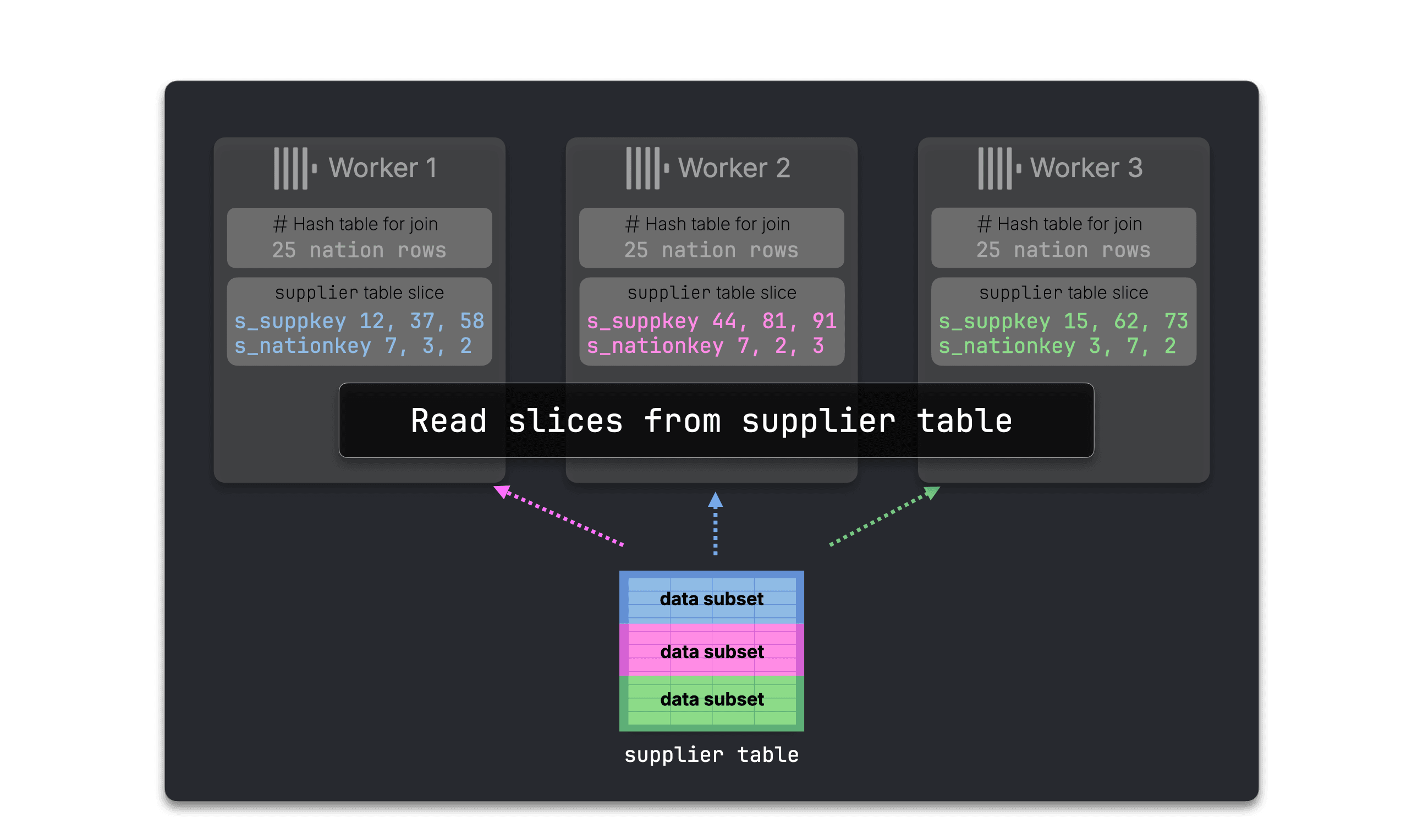 …and probes that local hash table.
The result is an enriched supplier ⋈ nation side.
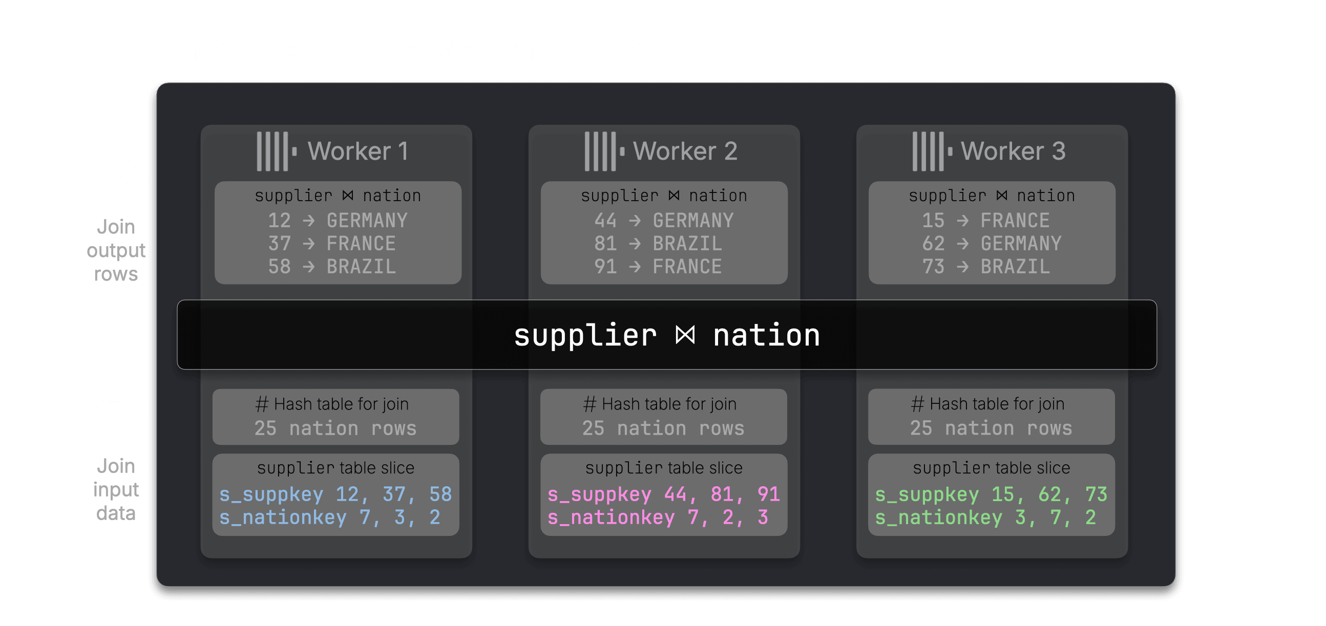
Nothing has been shuffled yet: each worker still keeps the rows from its original supplier slice.
Step 2: Co-locate lineitem with enriched supplier rows #
Next, ClickHouse prepares the larger join lineitem ⋈ (supplier ⋈ nation).
Workers first read slices of lineitem…
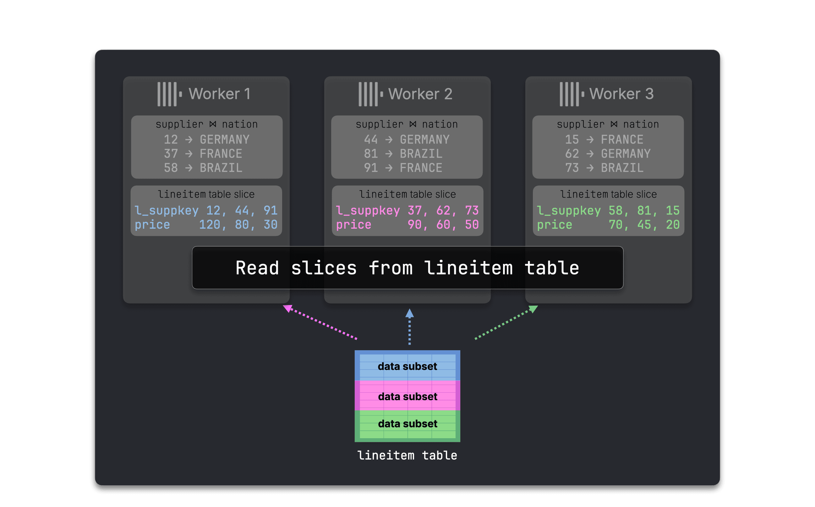
…and both join sides are repartitioned by supplier key: lineitem by l_suppkey, and the enriched supplier ⋈ nation rows by s_suppkey.
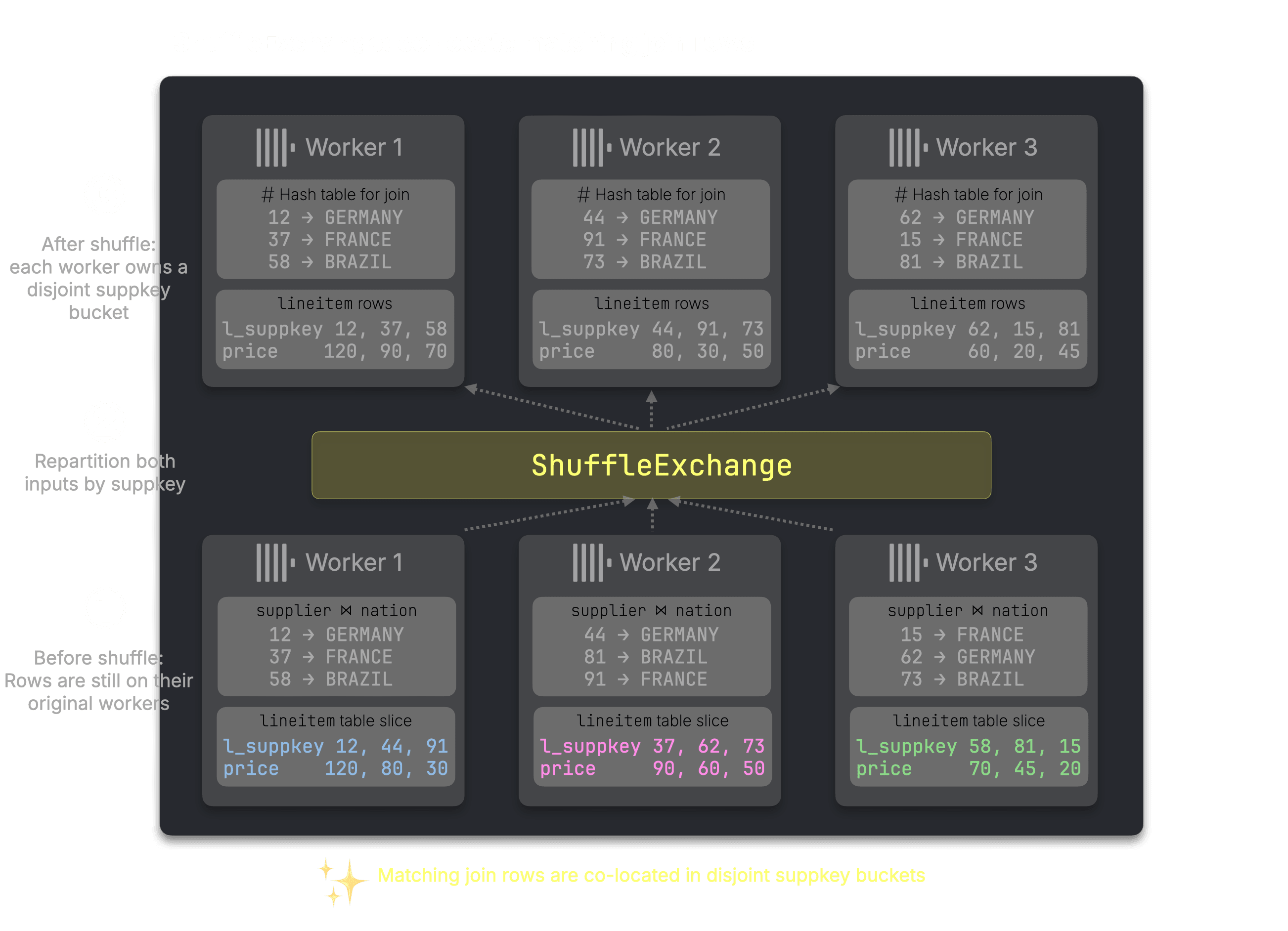
After the shuffle, each worker owns a disjoint supplier-key bucket containing the matching rows from both sides, and the enriched supplier ⋈ nation rows from Step 1 become the build side.
Prior bottleneck removed: no full build-side copy
Previously, each node needed the full right side of the join in memory. After the shuffle, each worker node owns only a disjoint supplier-key bucket, so it builds only its share of the hash table.
Step 3: Join locally within each supplier-key bucket #
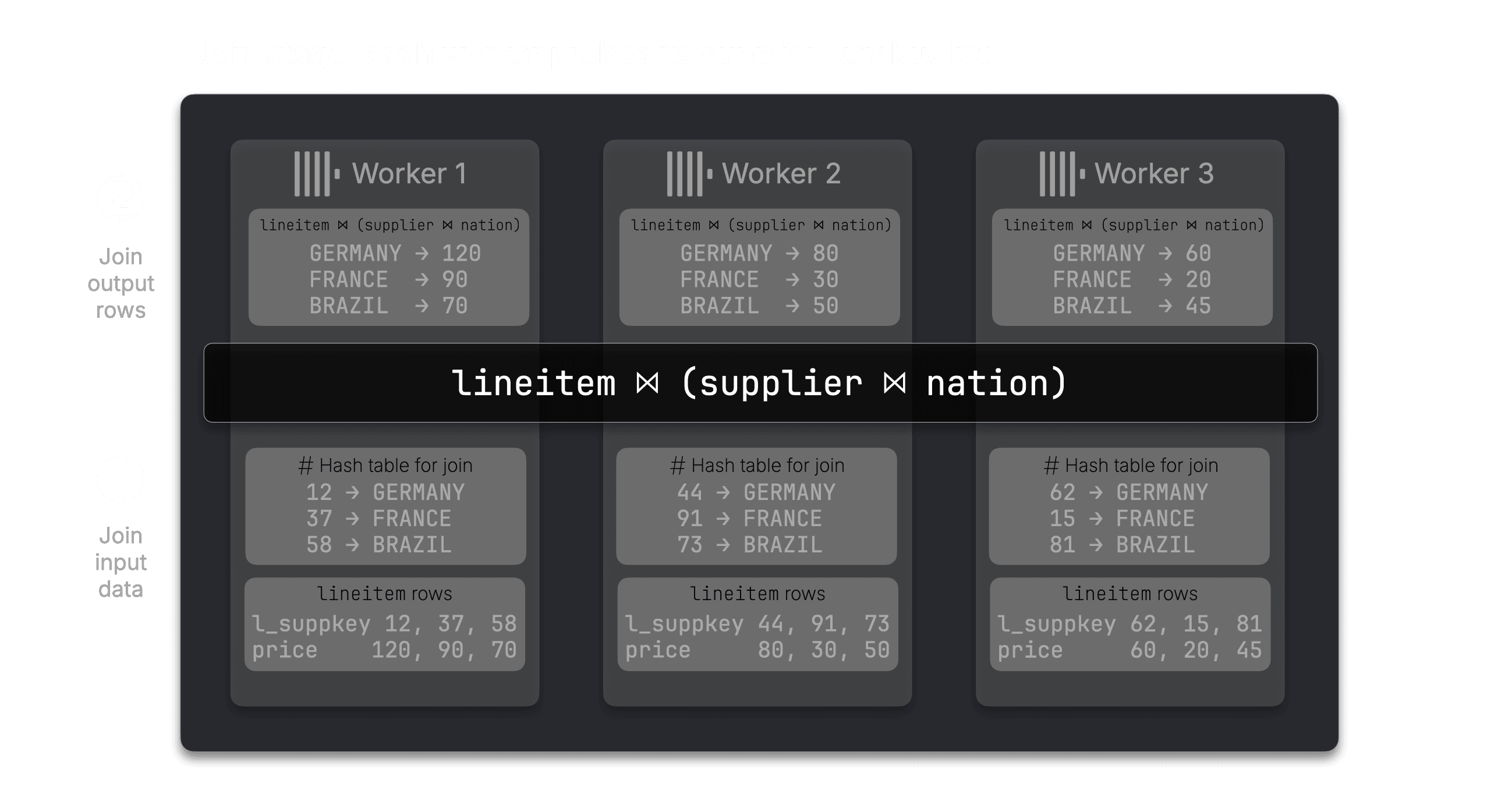
After the shuffle, each worker owns one supplier-key bucket. For that bucket, it has both sides of the join: matching lineitem rows and the enriched supplier ⋈ nation rows.
Each worker can now join locally by probing its bucket-local hash table. No worker needs the full build side, and no additional network exchange is needed for this join.
Step 4: Shuffle by GROUP BY key for final aggregation #
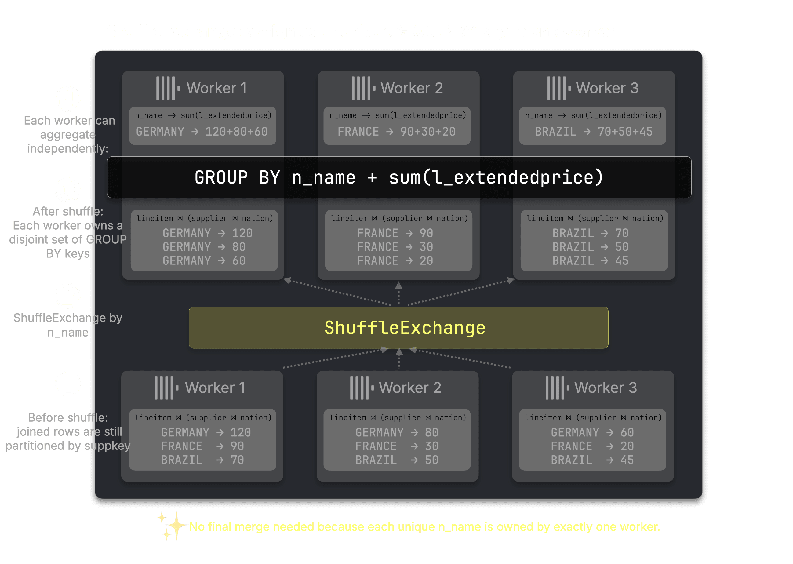
The join output is still partitioned by supplier key, not by n_name. So the same nation can appear on multiple workers. ClickHouse reshuffles the joined rows by the GROUP BY key, n_name, so each worker owns complete groups and can compute sum(l_extendedprice) independently.
Prior bottleneck removed: no single-node final aggregate merge
Previously, nodes could produce partial groups locally, but the same GROUP BY key could appear on multiple nodes, so one coordinator had to merge all partial states. After the shuffle by the GROUP BY key, each worker owns complete groups and can compute the final aggregate for its keys locally.
Here, n_name has only 25 distinct values, so the final merge would be small. But for high-cardinality GROUP BY, shuffling by the grouping key avoids the single-coordinator merge bottleneck. We’ll come back to this planning tradeoff at the end.
Step 5: Sort locally and gather the final result #
Each worker sorts its aggregated results by revenue. The GatherExchange (line 3) combines the sorted results from all workers at the coordinator to produce the final output.
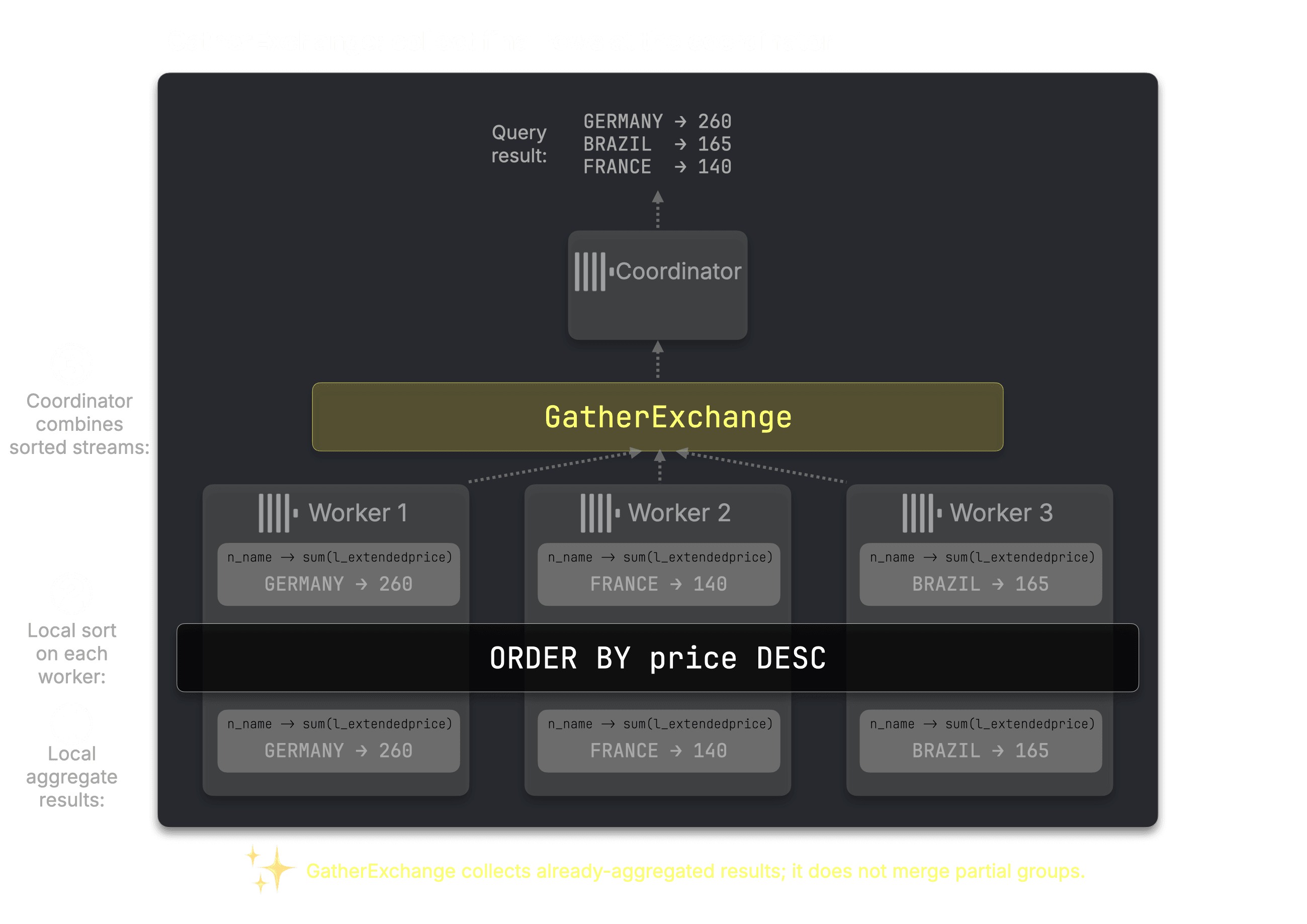
Prior bottleneck avoided: the coordinator only gathers final rows
The coordinator still receives the query result, but the expensive work has already happened across the workers. It gathers sorted, already-aggregated rows; it does not merge large partial groups or build a large join hash table.
The example above shows the logical data movement: shuffle here, broadcast there, gather at the end. Under the hood, ClickHouse Cloud needs a transport layer that can move those intermediate blocks efficiently between workers.
How does data move between stages? #
Exchanges can move data in two ways.
The default is streaming exchange. Workers send blocks directly to other workers over TCP using a custom binary protocol. Data starts moving as soon as it is produced: a worker reading lineitem can begin sending blocks into a ShuffleExchange immediately, while the receiving workers start consuming them without waiting for the full input. In other words, exchanges are pipelined rather than “write everything, then read everything.”
The second mode is persisted exchange. Instead of sending intermediate blocks directly between workers, ClickHouse writes them to shared object storage. This is useful for future fault recovery and for spilling intermediate results when a query exceeds cluster memory.
Streaming exchange is optimized for fast interactive queries and is the default. If a worker fails, the query fails and the client retries it. For these workloads, rerunning the query is usually cheaper than checkpointing every exchange.
Why ClickHouse Cloud makes this possible #
Multi-stage distributed execution depends on workers being interchangeable. A stage can run on any worker only if that worker can access the data and metadata it needs.
Shared storage makes workers interchangeable #
ClickHouse Cloud already has that foundation. Table data lives in shared object storage, and every node has access to the metadata needed to read it. The coordinator can therefore assign stages dynamically across the cluster: any worker can scan table data, receive shuffled rows, build its share of a hash table, aggregate its assigned groups, or sort its local result.
Shuffle improves memory utilization #
This also improves memory utilization. When a ShuffleExchange partitions a large join across 8 workers, each worker receives roughly 1/8 of the rows and builds roughly 1/8 of the hash table. A join that would require 16 GiB of memory on one node can instead use about 2 GiB per worker across 8 nodes.
Shared storage can avoid some broadcasts #
Shared storage also opens up future optimizations. For small tables, a worker may not need to receive a broadcast over the network at all; it can read the table directly from object storage and keep it in the local SSD cache for future reads. That is useful for dimension tables like nation or supplier, where local cached reads may be cheaper than broadcasting the table through the exchange layer.
Toward stateless workers #
The longer-term direction is fully stateless workers: nodes that can appear on demand, pick up work for a query, read the data they need from shared storage, and disappear again when the work is done. Without fixed ownership or manual data placement. Multi-stage distributed execution is a step toward that model.
What about single-node queries? #
ClickHouse’s single-node execution path is unchanged. Columnar MergeTree storage, vectorized execution, and aggressive pipeline parallelism are still the foundation of query performance.
Multi-stage distributed execution is an additional, opt-in path for queries that benefit from scaling across multiple nodes. It extends ClickHouse’s execution model and does not replace the single-node engine.
TPC-H benchmark results for multi-stage distributed query execution #
TPC-H is an industry-standard benchmark for analytical query processing. It consists of 22 queries across 8 tables, ranging from simple scans to complex multi-table joins, designed to simulate real-world decision-support workloads.
We ran it at scale factor 100 (~100GB of data), where the various tables have the following row counts:
lineitem(600M rows)orders(150M)partsupp(80M)part(20M)supplier(1M)nation(25)
We ran the benchmark on ClickHouse Cloud staging machines with ARM (Graviton), 8 cores, and 32 GB RAM. We’re using ClickHouse’s SharedMergeTree and server version 26.2.1.261
The table below shows the results from running each query on 1 node (our baseline) and 8 nodes using multi-stage distributed query execution. We run each query three times and take the best time.
| Query | 1 node | 8 nodes | Speedup | Notes |
|---|---|---|---|---|
| Q01 | 14.36s | 1.94s | 7.4x | Full scan + agg, near-linear |
| Q02 | 1.33s | 2.31s | 0.6x | Runtime filters are not fully supported |
| Q03 | 3.67s | 1.27s | 2.9x | 3-table join |
| Q04 | 3.13s | 0.74s | 4.2x | EXISTS subquery as join |
| Q05 | 6.16s | 2.31s | 2.7x | 6-table join |
| Q06 | 0.65s | 0.16s | 4.1x | Single-table scan |
| Q07 | 3.21s | 1.24s | 2.6x | 6-table join |
| Q08 | 5.61s | 2.65s | 2.1x | 8-table join |
| Q09 | 15.42s | 4.60s | 3.4x | 6-table join |
| Q10 | 5.90s | 2.39s | 2.5x | 4-table join |
| Q11 | 1.04s | 0.58s | 1.8x | 3-table join |
| Q12 | 2.45s | 0.81s | 3.0x | 2-table join |
| Q13 | 5.18s | 1.56s | 3.3x | 2-table join, two-level agg |
| Q14 | 0.49s | 0.21s | 2.3x | 2-table join |
| Q15 | 0.07s | 0.07s | 1.0x | Already fast |
| Q16 | 1.12s | 0.58s | 1.9x | 3-table join |
| Q17 | 5.99s | 2.88s | 2.1x | 2-table join + subquery |
| Q18 | 16.07s | 16.32s | 1.0x | EXISTS subquery not distributed by rule-based planner |
| Q19 | 8.09s | 1.78s | 4.5x | 2-table join |
| Q20 | 1.54s | 1.10s | 1.4x | 4-table join |
| Q21 | 14.83s | 8.77s | 1.7x | 4-table join with EXISTS/NOT EXISTS |
| Q22 | 1.31s | 0.38s | 3.4x | 2-table join |
| Total | 117.6s | 54.7s | 2.1x |
Why is Q02 slower? #
Some single-node optimizations are not yet fully supported in distributed mode, e.g., runtime filters (Bloom filter pushdowns across joins). Q02 shows a regression because of this.
What scales well? #
Near-linear scaling for scan-dominated queries.
Q01 (full scan + aggregation of 600M rows) achieves 7.4x on 8 nodes.
The work is almost entirely reading and aggregating, which splits evenly across workers with minimal exchange overhead.
Good scaling (2-5x) for multi-join queries.
Q19 (4.5x), Q04 (4.2x), Q06 (4.1x), Q09 (3.4x), Q22 (3.4x), Q13 (3.3x), Q12 (3.0x), Q03 (2.9x).
For these queries, there is significant shuffle overhead, as every exchange involves serializing data, network transfer, and deserialization, but it's proportionally small compared to the parallelized join computation.
Where is there room for smarter plans? #
The rule-based strategy works well for most queries, but some plans are suboptimal.
Q08 shuffles both sides of a join where one side has only 134K rows after filtering - a broadcast would save reshuffling 600M rows.
Q18's EXISTS subquery limits parallelism. Small tables like supplier (1M rows) are shuffled over the network even though every worker could read them directly from shared object storage.
These limitations are not fundamental to the execution engine. The engine can execute any plan it's given, the question is which plan to give it.
What’s next? #
We are working on a cost-based optimizer for multi-stage distributed query execution, which we expect will further improve query performance.
One important area is choosing the right aggregation strategy automatically. Some queries benefit from shuffling by the GROUP BY key so each worker owns complete groups; others are better served by local partial aggregation followed by a final merge. A cost-based optimizer can choose between these strategies based on cardinality, data size, and cluster shape.
Stay tuned for a future post.
How can I use multi-stage distributed query execution? #
At the time of writing (May 2026), multi-stage distributed execution is experimental and only available in ClickHouse Cloud as part of a private preview program.
To request access, reach out to your ClickHouse account team or contact us at support@clickhouse.com