ClickHouse Release 25.10

Another month goes by, which means it’s time for another release!

ClickHouse version 25.10 contains 20 new features 👻 30 performance optimizations 🔮 103 bug fixes 🎃

This release introduces a collection of join improvements, a new data type for vector search, late materialization of secondary indices, and more!

New contributors #

A special welcome to all the new contributors in 25.10! The growth of ClickHouse's community is humbling, and we are always grateful for the contributions that have made ClickHouse so popular.

Below are the names of the new contributors:

0xgouda, Ahmed Gouda, Albert Chae, Austin Bonander, ChaiAndCode, David E. Wheeler, DeanNeaht, Dylan, Frank Rosner, GEFFARD Quentin, Giampaolo Capelli, Grant Holly, Guang, Guang Zhao, Isak Ellmer, Jan Rada, Kunal Gupta, Lonny Kapelushnik, Manuel Raimann, Michal Simon, Narasimha Pakeer, Neerav, Raphaël Thériault, Rui Zhang, Sadra Barikbin, copilot-swe-agent[bot], dollaransh17, flozdra, jitendra1411, neeravsalaria, pranav mehta, zlareb1, |2ustam, Андрей Курганский, Артем Юров

Hint: if you’re curious how we generate this list… here.

You can also view the slides from the presentation.

Lazy columns replication in JOINs #

Contributed by Pavel Kruglov #

"When will you stop optimizing join performance?"
We will never stop!

This release once again brings JOIN performance optimizations.

The first join improvement in 25.10 is lazy columns replication, a new optimization that reduces CPU and memory usage when JOINs produce many duplicate values.

When running JOIN queries (including those using the arrayJoin function), values from the input tables are often replicated in the result, especially when there are many matches for a given key.

As an example, consider a hits table containing anonymized web analytics data, sketched below with two columns, ClientIP and URL:

When we run a self-join:

1SELECT ...
2FROM
3    hits AS t1 INNER JOIN hits AS t2
4    ON t1.ClientIP = t2.ClientIP;

Then the result can heavily duplicate values from both sides:

For large columns (like URL), this replication consumes significant CPU cycles and memory, as the same values are repeatedly copied in memory.

With 25.10, ClickHouse no longer spends CPU and memory replicating identical values during JOINs.

Instead, we’ve introduced a new internal representation for replicated columns like URL.

Rather than physically replicating data, ClickHouse now keeps the original non-replicated column alongside a compact index column that points to it:

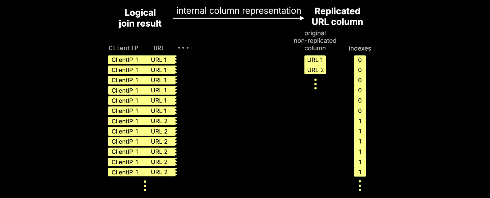
We call this mechanism lazy columns replication; it defers physical value replication until it’s actually needed (and often, it never is).

To control this behavior, use the settings

• enable_lazy_columns_replication
• allow_special_serialization_kinds_in_output_formats

Inspecting the effect in practice #

To measure the effect, we benchmarked this feature on an AWS EC2 m6i.8xlarge instance (32 vCPUs, 128 GiB RAM) using the hits table.

Here is how you can create and load this table on your own.

First, we ran the example self-join without lazy replication:

1SELECT sum(cityHash64(URL))
2FROM
3    hits AS t1 INNER JOIN hits AS t2
4    ON t1.ClientIP = t2.ClientIP
5SETTINGS
6    enable_lazy_columns_replication = 0,
7    allow_special_serialization_kinds_in_output_formats = 0;

┌─sum(cityHash64(URL))─┐
│  8580639250520379278 │
└──────────────────────┘

1 row in set. Elapsed: 83.396 sec. Processed 199.99 million rows, 10.64 GB (2.40 million rows/s., 127.57 MB/s.)
Peak memory usage: 4.88 GiB.

Then, we ran the same query with lazy columns replication enabled:

1SELECT sum(cityHash64(URL))
2FROM
3    hits AS t1 INNER JOIN hits AS t2
4    ON t1.ClientIP = t2.ClientIP
5SETTINGS
6    enable_lazy_columns_replication = 1,
7    allow_special_serialization_kinds_in_output_formats = 1;

┌─sum(cityHash64(URL))─┐
│  8580639250520379278 │
└──────────────────────┘

1 row in set. Elapsed: 4.078 sec. Processed 199.99 million rows, 10.64 GB (49.04 million rows/s., 2.61 GB/s.)
Peak memory usage: 4.57 GiB.

Result: “Lazy columns replication” made this self-join over 20× faster while slightly reducing peak memory use, by avoiding unnecessary copying of large string values.

Bloom filters in JOINs #

Contributed by Alexander Gololobov #

The next join optimization generalizes a technique already used in ClickHouse’s full sorting merge join algorithm, where joined tables can be filtered by each other’s join keys before the actual join takes place.

In 25.10, a similar optimization has been introduced for ClickHouse’s fastest join algorithm, the parallel hash join.

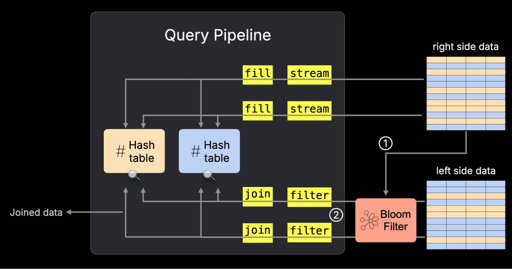
The join is sped up by ① building a bloom filter from the join’s right side join key data at runtime and passing this filter to the ② scan in the join’s left side data. The diagram below sketches this for the parallel hash join’s physical query plan (“query pipeline”). You can read how the rest of this plan works here.

This optimization is controlled by the setting enable_join_runtime_filters.

We benchmarked this feature on an AWS EC2 m6i.8xlarge instance (32 vCPUs, 128 GiB RAM) using the TPC-H dataset with scale factor 100. Below, we’ll first inspect how the optimization changes the query plan, and then measure its impact in practice.

Inspecting the logical plan #

The easiest way to look under the hood of a JOIN query is by inspecting its logical query plan with EXPLAIN plan.

Let’s do that for a simple join between the TPC-H orders and customer tables on the custkey column, where we disabled the bloom filter based pre-filtering:

1EXPLAIN plan
2SELECT *
3FROM orders, customer
4WHERE o_custkey = c_custkey
5SETTINGS enable_join_runtime_filters = 0;

The relevant part of the plan looks like this:

...                             
Join                                                       
...
ReadFromMergeTree (default.orders)                   
ReadFromMergeTree (default.customer)

We’ll skip the rest of the plan and focus on the core mechanics.

Reading the output from bottom to top, we can see that ClickHouse plans to read the data from the two tables, orders and customer, and perform the join.

Next, let’s inspect the logical query plan for the same join, but this time with runtime pre-filtering enabled:

1EXPLAIN plan
2SELECT *
3FROM orders, customer
4WHERE o_custkey = c_custkey
5SETTINGS enable_join_runtime_filters = 1;

The relevant parts of the plan look like this:

...
Join                                                                                                                                                                                             
...                                                                                                                                                                         
Prewhere filter column: __filterContains(_runtime_filter_14211390369232515712_0, __table1.o_custkey)                                                                          
...
BuildRuntimeFilter (Build runtime join filter on __table2.c_custkey (_runtime_filter_14211390369232515712_0))
...

Reading the plan from bottom to top, we can see that ClickHouse first ① builds a Bloom filter from the join key values on the right-hand side (customer) table.

This runtime filter is then ② applied as a PREWHERE filter on the left-hand side (orders) table, allowing irrelevant rows to be skipped before the join is executed.

Running the query with and without runtime filtering #

Now let’s actually run a slightly extended version of that join query, this time joining orders, customer, and nation, and calculating the average order total for customers from France.

We’ll start with runtime pre-filtering disabled:

1SELECT avg(o_totalprice)
2FROM orders, customer, nation
3WHERE (c_custkey = o_custkey) AND (c_nationkey = n_nationkey) AND (n_name = 'FRANCE')
4SETTINGS enable_join_runtime_filters = 0;

┌──avg(o_totalprice)─┐
│ 151149.41468432106 │
└────────────────────┘

1 row in set. Elapsed: 1.005 sec. Processed 165.00 million rows, 1.92 GB (164.25 million rows/s., 1.91 GB/s.)
Peak memory usage: 1.24 GiB.

Then, we run the same query again, this time with runtime pre-filtering enabled:

1SELECT avg(o_totalprice)
2FROM orders, customer, nation
3WHERE (c_custkey = o_custkey) AND (c_nationkey = n_nationkey) AND (n_name = 'FRANCE')
4SETTINGS enable_join_runtime_filters = 1;

┌──avg(o_totalprice)─┐
│ 151149.41468432106 │
└────────────────────┘

1 row in set. Elapsed: 0.471 sec. Processed 165.00 million rows, 1.92 GB (350.64 million rows/s., 4.08 GB/s.)
Peak memory usage: 185.18 MiB.

Result:

With runtime pre-filtering enabled, the same query ran 2.1× faster while using nearly 7× less memory.

By filtering rows early with Bloom filters, ClickHouse avoids scanning and processing unnecessary data, delivering faster joins and lower resource usage.

Push-down of complex conditions in JOINs #

Contributed by Yarik Briukhovetskyi #

ClickHouse can now push down complex OR conditions in JOIN queries to filter each table earlier, before the join actually happens.

This optimization works when every branch of an OR condition includes at least one filter (predicate) for each table involved in the join.

For example:

1(t1.k IN (1,2) AND t2.x = 100)
2OR
3(t1.k IN (3,4) AND t2.x = 200)

In this case, both sides of the join (t1 and t2) have predicates in every branch.

ClickHouse can therefore combine and push them down as:

• t1.k IN (1,2,3,4) for the left table

• t2.x IN (100,200) for the right table

This allows both tables to be pre-filtered before the join, reducing the data read and improving performance.

This optimization is available under the setting use_join_disjunctions_push_down.

To see how this optimization works in practice, we’ll look at a simple example using the TPC-H dataset (scale factor 100) on an AWS EC2 m6i.8xlarge instance (32 vCPUs, 128 GiB RAM).

We’ll join the customer and nation tables on c_nationkey, using a condition that contains two OR branches, each filtering both sides of the join.

Inspecting the logical plan #

First, let’s inspect the logical query plan for this query without the push-down optimization:

1EXPLAIN plan
2SELECT *
3FROM customer AS c
4INNER JOIN nation AS n
5    ON c.c_nationkey = n.n_nationkey
6WHERE (c.c_name LIKE 'Customer#00000%' AND n.n_name = 'GERMANY')
7   OR (c.c_name LIKE 'Customer#00001%' AND n.n_name = 'FRANCE')
8SETTINGS use_join_disjunctions_push_down = 0;

In this plan, ClickHouse simply reads data from both tables and applies the full filter during the join:

Join                                                       
...
ReadFromMergeTree (default.customer)
ReadFromMergeTree (default.nation)

Now, let’s enable the new optimization:

1EXPLAIN plan
2SELECT *
3FROM customer AS c
4INNER JOIN nation AS n
5    ON c.c_nationkey = n.n_nationkey
6WHERE (c.c_name LIKE 'Customer#00000%' AND n.n_name = 'GERMANY')
7   OR (c.c_name LIKE 'Customer#00001%' AND n.n_name = 'FRANCE')
8SETTINGS use_join_disjunctions_push_down = 1;

This time, ClickHouse identifies that both branches contain predicates for both tables.

It derives separate filters for each side, pushing them down so that both customer and nation are filtered before the join:

Join
...
Filter
ReadFromMergeTree (default.customer)
...
Filter
ReadFromMergeTree (default.nation)

Benchmarking the effect #

Next, let’s actually run the query with the optimization disabled and enabled to see the performance difference.

Without push-down:

1SELECT *
2FROM customer AS c
3INNER JOIN nation AS n
4    ON c.c_nationkey = n.n_nationkey
5WHERE (c.c_name LIKE 'Customer#00000%' AND n.n_name = 'GERMANY')
6   OR (c.c_name LIKE 'Customer#00001%' AND n.n_name = 'FRANCE')
7SETTINGS use_join_disjunctions_push_down = 0;

788 rows in set. Elapsed: 0.240 sec. Processed 15.00 million rows, 2.93 GB (62.56 million rows/s., 12.21 GB/s.)
Peak memory usage: 261.30 MiB.

With push-down enabled:

1SELECT *
2FROM customer AS c
3INNER JOIN nation AS n
4    ON c.c_nationkey = n.n_nationkey
5WHERE (c.c_name LIKE 'Customer#00000%' AND n.n_name = 'GERMANY')
6   OR (c.c_name LIKE 'Customer#00001%' AND n.n_name = 'FRANCE')
7SETTINGS use_join_disjunctions_push_down = 0;

788 rows in set. Elapsed: 0.010 sec. Processed 24.60 thousand rows, 4.81 MB (2.47 million rows/s., 482.53 MB/s.)
Peak memory usage: 4.30 MiB.

Result:

With push-down enabled, the same query ran 24× faster and used over 60× less memory.

By pushing filters for both sides of the join down to the table scan, ClickHouse avoids reading and processing millions of irrelevant rows.

Automatically build column statistics for MergeTree tables #

Contributed by Anton Popov #

This is the fourth join-related optimization in this release, albeit an indirect one.

In the previous release, ClickHouse introduced automatic global join reordering, allowing the engine to efficiently reorder complex join graphs spanning dozens of tables. This resulted in significant improvements, for example, a 1,450x speedup and 25× reduction in memory usage on one TPC-H example query.

Global join reordering works best when column statistics are available for the join keys and filters involved. Until now, these statistics had to be created manually for each column.

Starting with 25.10, ClickHouse can now automatically create statistics for all suitable columns in a MergeTree table using the new table-level setting auto_statistics_types.

This setting defines which types of statistics to build (for example, minmax, uniq, countmin):

1CREATE TABLE tpch.orders (...) ORDER BY (o_orderkey)
2SETTINGS auto_statistics_types = 'minmax, uniq, countmin';

This enables statistics generation for all columns in the table automatically.

You can also configure it globally for all MergeTree tables in your server configuration:

1$ cat /etc/config.d/merge_tree.yaml

merge_tree:
    auto_statistics_types: 'minmax, uniq, countmin'

By keeping statistics up to date automatically, ClickHouse can make smarter join and filter decisions, improving query planning and reducing both memory use and runtime without manual tuning.

These four features (lazy columns replication, bloom filters in JOINs, push-down of complex conditions, and automatic column statistics) are the latest in a long line of JOIN optimizations in ClickHouse, and they won’t be the last.

QBit data type #

Contributed by Raufs Dunamalijevs #

QBit is a data type for vector embeddings that lets you tune search precision at runtime. It uses a bit-sliced data layout where every number is sliced by bits, and at query time, we specify, how many (most significant) bits to take.

1CREATE TABLE vectors (
2    id UInt64, name String, ...
3    vec QBit(BFloat16, 1536)
4) ORDER BY ();

1SELECT id, name FROM vectors
2ORDER BY L2DistanceTransposed(vector, target, 10)
3LIMIT 10;

Raufs Dunamalijevs has written in detail about the QBit in the blog post ‘We built a vector search engine that lets you choose precision at query time’.

SQL updates #

Contributed by Nihal Z. Miaji, Surya Kant Ranjan, Simon Michal #

The ClickHouse 25.10 release sees several additions to the supported SQL syntax.

First up is general support for the <=> (IS NOT DISTINCT FROM) operator, which was previously only supported in the JOIN ON part of a query. This operator offers equality comparison that treats NULLs as identical. Let’s have a look at how it works:

1SELECT NULL <=> NULL, NULL = NULL;

┌─isNotDistinc⋯NULL, NULL)─┬─equals(NULL, NULL)─┐
│                        1 │ ᴺᵁᴸᴸ               │
└──────────────────────────┴────────────────────┘

Next up, we have negative limit and offset. This is useful for a query where we want to retrieve the n most recent records, but return them in ascending order. Let’s explore this feature using the UK property prices dataset.

Imagine we want to find properties sold for over £10 million since 2024, in descending date order. We could write the following query:

1SELECT date, price, county, district
2FROM uk.uk_price_paid
3WHERE date >= '2024-01-01' AND price > 10_000_000
4ORDER BY date DESC LIMIT 10;

┌───────date─┬────price─┬─county────────────────────┬─district──────────────────┐
│ 2025-03-13 │ 12000000 │ CHESHIRE WEST AND CHESTER │ CHESHIRE WEST AND CHESTER │
│ 2025-03-06 │ 18375000 │ STOKE-ON-TRENT            │ STOKE-ON-TRENT            │
│ 2025-03-06 │ 10850000 │ HERTFORDSHIRE             │ HERTSMERE                 │
│ 2025-03-04 │ 11000000 │ PORTSMOUTH                │ PORTSMOUTH                │
│ 2025-03-04 │ 18000000 │ GREATER LONDON            │ HAMMERSMITH AND FULHAM    │
│ 2025-03-03 │ 12500000 │ ESSEX                     │ BASILDON                  │
│ 2025-02-20 │ 16830000 │ GREATER LONDON            │ CITY OF WESTMINSTER       │
│ 2025-02-13 │ 13950000 │ GREATER LONDON            │ KENSINGTON AND CHELSEA    │
│ 2025-02-07 │ 81850000 │ ESSEX                     │ EPPING FOREST             │
│ 2025-02-07 │ 24920000 │ GREATER LONDON            │ HARINGEY                  │
└────────────┴──────────┴───────────────────────────┴───────────────────────────┘

But let’s say we want to get those same most recent 10 sales, but have them sorted in ascending order by date. This is where negative limit functionality comes in handy. We can adjust the ORDER BY and LIMIT parts of the query like so:

1SELECT date, price, county, district
2FROM uk.uk_price_paid
3WHERE date >= '2024-01-01' AND price > 10_000_000
4ORDER BY date LIMIT -10;

And then we’ll see the following results:

┌───────date─┬────price─┬─county────────────────────┬─district──────────────────┐
│ 2025-02-07 │ 29240000 │ GREATER LONDON            │ MERTON                    │
│ 2025-02-07 │ 75960000 │ WARRINGTON                │ WARRINGTON                │
│ 2025-02-13 │ 13950000 │ GREATER LONDON            │ KENSINGTON AND CHELSEA    │
│ 2025-02-20 │ 16830000 │ GREATER LONDON            │ CITY OF WESTMINSTER       │
│ 2025-03-03 │ 12500000 │ ESSEX                     │ BASILDON                  │
│ 2025-03-04 │ 11000000 │ PORTSMOUTH                │ PORTSMOUTH                │
│ 2025-03-04 │ 18000000 │ GREATER LONDON            │ HAMMERSMITH AND FULHAM    │
│ 2025-03-06 │ 18375000 │ STOKE-ON-TRENT            │ STOKE-ON-TRENT            │
│ 2025-03-06 │ 10850000 │ HERTFORDSHIRE             │ HERTSMERE                 │
│ 2025-03-13 │ 12000000 │ CHESHIRE WEST AND CHESTER │ CHESHIRE WEST AND CHESTER │
└────────────┴──────────┴───────────────────────────┴───────────────────────────┘

We can also provide a negative offset alongside a negative limit to paginate through results. To see the next 10 most recent sales sorted in ascending order by date, we can write the following query:

1SELECT date, price, county, district
2FROM uk.uk_price_paid
3WHERE date >= '2024-01-01' AND price > 10_000_000
4ORDER BY date LIMIT -10 OFFSET -10;

┌───────date─┬─────price─┬─county──────────┬─district────────────┐
│ 2025-01-21 │  10650000 │ NOTTINGHAMSHIRE │ ASHFIELD            │
│ 2025-01-21 │  22722671 │ GREATER LONDON  │ CITY OF WESTMINSTER │
│ 2025-01-22 │ 109500000 │ GREATER LONDON  │ CITY OF LONDON      │
│ 2025-01-24 │  11700000 │ THURROCK        │ THURROCK            │
│ 2025-01-25 │  75570000 │ GREATER LONDON  │ CITY OF WESTMINSTER │
│ 2025-01-29 │  12579711 │ SUFFOLK         │ MID SUFFOLK         │
│ 2025-01-31 │  29307333 │ GREATER LONDON  │ EALING              │
│ 2025-02-07 │  81850000 │ ESSEX           │ EPPING FOREST       │
│ 2025-02-07 │  24920000 │ GREATER LONDON  │ HARINGEY            │
│ 2025-02-07 │ 151420000 │ GREATER LONDON  │ MERTON              │
└────────────┴───────────┴─────────────────┴─────────────────────┘

And if we wanted to get the next 10, we’d change the last line of the query to say LIMIT -10 OFFSET -20, and so on.

Finally, ClickHouse now supports LIMIT BY ALL. Let’s have a look at an example where we can use this clause. The following query returns information about residential properties sold for more than £10 million in Greater London:

1SELECT town, district, type
2FROM uk.uk_price_paid
3WHERE county = 'GREATER LONDON' AND price > 10_000_000 AND type <> 'other'
4ORDER BY price DESC
5LIMIT 10;

┌─town───┬─district───────────────┬─type─────┐
│ LONDON │ CITY OF WESTMINSTER    │ flat     │
│ LONDON │ CITY OF WESTMINSTER    │ flat     │
│ LONDON │ CITY OF WESTMINSTER    │ flat     │
│ LONDON │ CITY OF WESTMINSTER    │ flat     │
│ LONDON │ CITY OF WESTMINSTER    │ flat     │
│ LONDON │ CITY OF WESTMINSTER    │ terraced │
│ LONDON │ CITY OF WESTMINSTER    │ flat     │
│ LONDON │ KENSINGTON AND CHELSEA │ terraced │
│ LONDON │ CITY OF WESTMINSTER    │ terraced │
│ LONDON │ KENSINGTON AND CHELSEA │ flat     │
└────────┴────────────────────────┴──────────┘

The City of Westminster has been returned many times, which makes sense, as it’s a costly part of the city. Let’s say we only want to return each combination of (town,district,type) once. We could do this using the LIMIT BY syntax:

1SELECT town, district, type
2FROM uk.uk_price_paid
3WHERE county = 'GREATER LONDON' AND price > 10_000_000 AND type <> 'other'
4ORDER BY price DESC
5LIMIT 1 BY town, district, type
6LIMIT 10;

┌─town───┬─district───────────────┬─type──────────┐
│ LONDON │ CITY OF WESTMINSTER    │ flat          │
│ LONDON │ CITY OF WESTMINSTER    │ terraced      │
│ LONDON │ KENSINGTON AND CHELSEA │ terraced      │
│ LONDON │ KENSINGTON AND CHELSEA │ flat          │
│ LONDON │ KENSINGTON AND CHELSEA │ detached      │
│ LONDON │ SOUTHWARK              │ flat          │
│ LONDON │ KENSINGTON AND CHELSEA │ semi-detached │
│ LONDON │ CITY OF WESTMINSTER    │ detached      │
│ LONDON │ CAMDEN                 │ detached      │
│ LONDON │ CITY OF LONDON         │ detached      │
└────────┴────────────────────────┴───────────────┘

Alternatively, instead of having to list all field names after the LIMIT BY, we use LIMIT BY ALL:

1SELECT town, district, type
2FROM uk.uk_price_paid
3WHERE county = 'GREATER LONDON' AND price > 10_000_000 AND type <> 'other'
4ORDER BY price DESC
5LIMIT 1 BY ALL
6LIMIT 10;

And we’ll get back the same set of records.

Arrow Flight server and client compatibility #

Contributed by zakr600, Vitaly Baranov #

In ClickHouse 25.8, we introduced the Arrow Flight integration, which made it possible to use ClickHouse as an Arrow Flight server or client.

The integration was initially quite rudimentary, but it has been developed over the last couple of months. As of ClickHouse 25.10, we can query the ClickHouse Arrow Flight server using the ClickHouse Arrow Flight client.

We can add a config file containing the following to our ClickHouse Server:

1arrowflight_port: 6379
2arrowflight:
3  enable_ssl: false
4  auth_required: false

We’ll then have an Arrow Flight Server running on port 6379. At the moment, you can only query the default database, but we can use the new alias table engine to work around this:

1CREATE TABLE uk_price_paid
2ENGINE = Alias(uk, uk_price_paid);

And then we can query that table using our Arrow client:

1SELECT max(price), count()
2FROM arrowflight('localhost:6379', 'uk_price_paid', 'default', '');

┌─max(price)─┬──count()─┐
│  900000000 │ 30452463 │
└────────────┴──────────┘

Late materialization of secondary indices #

Contributed by George Larionov #

The 25.10 release also introduces settings that allow us to delay the materialization of secondary indices. We might want to do this if we have tables that contain indices that take a while to populate (e.g., the approximate vector search index).

Let’s see how this works with help from some DBpedia embeddings. We’ll ingest them into the following table:

1CREATE OR REPLACE TABLE dbpedia
2(
3  id      String,
4  title   String,
5  text    String,
6  vector  Array(Float32) CODEC(NONE),
7  INDEX vector_idx vector TYPE vector_similarity('hnsw', 'L2Distance', 1536)
8) ENGINE = MergeTree
9ORDER BY (id);

We’ll then download one Parquet file that contains around 40,000 embeddings:

1wget https://huggingface.co/api/datasets/Qdrant/dbpedia-entities-openai3-text-embedding-3-large-1536-1M/parquet/default/train/0.parquet

Now let’s insert those records into our table:

1INSERT INTO dbpedia
2SELECT `_id` AS id, title, text, 
3       `text-embedding-3-large-1536-embedding` AS vector
4FROM file('0.parquet');

0 rows in set. Elapsed: 6.161 sec. Processed 38.46 thousand rows, 367.26 MB (6.24 thousand rows/s., 59.61 MB/s.)
Peak memory usage: 932.41 MiB.

It takes just over 6 seconds to ingest the records, while also materializing the HNSW index.

Let’s now create a copy of the dbpedia table:

1create table dbpedia2 as dbpedia;

We can now choose to delay the point at which index materialization happens by configuring the following setting:

1SET exclude_materialize_skip_indexes_on_insert='vector_idx';

If we repeat our earlier insert statement, but on dbpedia2:

1INSERT INTO dbpedia2
2SELECT `_id` AS id, title, text, 
3       `text-embedding-3-large-1536-embedding` AS vector
4FROM file('0.parquet');

We can see it’s significantly quicker:

0 rows in set. Elapsed: 0.522 sec. Processed 38.46 thousand rows, 367.26 MB (73.68 thousand rows/s., 703.59 MB/s.)
Peak memory usage: 931.08 MiB.

We can see whether the index has been materialized by writing the following query:

1SELECT table, data_compressed_bytes, data_uncompressed_bytes, marks_bytes FROM system.data_skipping_indices
2WHERE name = 'vector_idx';

┌─table────┬─data_compressed_bytes─┬─data_uncompressed_bytes─┬─marks_bytes─┐
│ dbpedia  │             124229003 │               128770836 │          50 │
│ dbpedia2 │                     0 │                       0 │           0 │
└──────────┴───────────────────────┴─────────────────────────┴─────────────┘

In dbpedia2, we can see that the number of bytes taken is 0, which is what we’d expect. The index will be materialized in the background merge process, but if we want to make it happen immediately, we can run this query:

1ALTER TABLE dbpedia2 MATERIALIZE INDEX vector_idx 
2SETTINGS mutations_sync = 2;

Re-running the query against the data_skipping_indices table will return the following output:

┌─table────┬─data_compressed_bytes─┬─data_uncompressed_bytes─┬─marks_bytes─┐
│ dbpedia  │             124229003 │               128770836 │          50 │
│ dbpedia2 │             124237137 │               128769912 │          50 │
└──────────┴───────────────────────┴─────────────────────────┴─────────────┘

Alternatively, we can query the system.parts table if we want to see whether any indices have been materialized for a given part:

1SELECT name, table, secondary_indices_compressed_bytes, secondary_indices_uncompressed_bytes, secondary_indices_marks_bytes 
2FROM system.parts;

Row 1:
──────
name:                                 all_1_1_0
table:                                dbpedia
secondary_indices_compressed_bytes:   124229003 -- 124.23 million
secondary_indices_uncompressed_bytes: 128770836 -- 128.77 million
secondary_indices_marks_bytes:        50

Row 2:
──────
name:                                 all_1_1_0_2
table:                                dbpedia2
secondary_indices_compressed_bytes:   124237137 -- 124.24 million
secondary_indices_uncompressed_bytes: 128769912 -- 128.77 million
secondary_indices_marks_bytes:        50

We can even disable building indices during merges by using the following setting:

1CREATE TABLE t (...)
2SETTINGS materialize_skip_indexes_on_merge = false;

Or exclude certain (heavy) indices from calculation:

1CREATE TABLE t (...)
2SETTINGS exclude_materialize_skip_indexes_on_merge = 'vector_idx';